Benchmarking and Scaling

Overview

Teaching: 30 min
Exercises: 15 min

Questions

• What is benchmarking?

• How do I do a benchmark?

• What is scaling?

• How do I perform a scaling analysis?

Objectives

• Be able to perform a benchmark analysis of an application

• Be able to perform a scaling analysis of an application

• Understand what good scaling performance looks like

What is benchmarking?

To get an idea of what we mean by benchmarking, let’s take the example of a sprint athlete. The athlete runs a predetermined distance on a particular surface, and a time is recorded. Based on different conditions, such as how dry or wet the surface is, or what the surface is made of (grass, sand, or track) the times of the sprinter to cover a distance (100m, 200m, 400m etc) will differ. If you know where the sprinter is running, and what the conditions were like, when the sprinter sets a certain time you can cross-correlate it with the known times associated with certain surfaces (our benchmarks) to judge how well they are performing.

Benchmarking in computing works in a similar way: it is a way of assessing the performance of a program (or set of programs), and benchmark tests are designed to mimic a particular type of workload on a component or system. They can also be used to measure differing performance across different systems. Usually codes are tested on different computer architectures to see how a code performs on each one. Like our sprinter, the times of benchmarks depends on a number of things: software, hardware or the computer itself and it’s architecture.

Callout: Local vs system-wide installations

Whenever you get access to an HPC system, there are usually two ways to get access to software: either you use a system-wide installation or you install it yourself. For widely used applications, it is likely that you should be able to find a system-wide installation. In many cases using the system-wide installation is the better option since the system administrators will (hopefully) have configured the application to run optimally for that system. If you can’t easily find your application, contact user support for the system to help you.

For less widely used codes, such as HemeLB, you will have to compile the code on the HPC system for your own use. Build scripts are available to help streamline this process but these must be customised to the specific libraries and nomenclature of individual HPC systems.

In either case, you should still check the benchmark case though! Sometimes system administrators are short on time or background knowledge of applications and do not do thorough testing. For locally compiled codes, the default options for compilers and libraries may not necessarily be optimal for performance. Benchmark testing can allow the best option for that machine to be identified.

The ideal benchmarking study

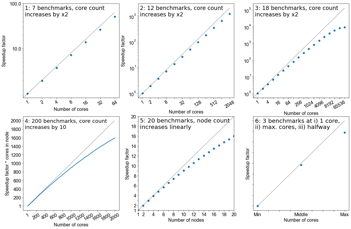
Benchmarking is a process that judges how well a piece of software runs on a system. Based on what you have learned thus far from running your own benchmarks, which of the following would represent a good benchmarking analysis?

1. 7 benchmarks, core count increases by factor of 2
2. 12 benchmarks, core count increases by factor of 2
3. 18 benchmarks, core count increases by factor of 2
4. 200 benchmarks, core count increases by 10
5. 20 benchmarks, node count increases linearly
6. 3 benchmarks; i) 1 core, ii) the maximum of cores possible, iii) a point at halfway

Solution

1. No, the core counts that are being benchmarked are too low and the number of points is not sufficient
2. Yes, but depends on the software you are working with, how you want to use it, and how big your system is. This does not give a true view how scalable it is at higher core counts.
3. Yes. If the system allows it and you have more cores at your disposal, this is the ideal benchmark to run. But as with #2, it depends on how you wish to utlise the software.
4. No, although it increases by a factor of 10 to 2000 cores, there are too many points on the graph and therefore would be highly impractical. Benchmarks are used to get an idea of scalability, the exact performance will vary with every benchmark run.
5. Yes. This is also a suitable metric for benchmarking, similar to response #3.
6. No. While this will cover the spread of simulation possibilities on the machine, it will be too sparse to permit an appropriate characterisation of the the code on your system. Depending on the operational restrictions of your system, full machine jobs may not be possible to run or may require a long time before it launches.

Creating a job file

HPC systems typically use a job scheduler to manage the deployment of jobs and their many different resource requests from multiple users. Common examples of schedulers include SLURM and PBS.

We will now work on creating a job file which we can run on SuperMUC-NG. Writing a job file from scratch is error prone, and most supercomputing centres will have a basic one which you can modify. Below is a job file we can use and modify for the rest of the course.

#!/bin/bash
# Job Name and Files
#SBATCH -J jobname

#Output and error:
#SBATCH -o ./%x.%j.out
#SBATCH -e ./%x.%j.err
#Initial working directory:
#SBATCH -D ./

# Wall clock limit:
#SBATCH --time=00:15:00

#Setup of execution environment
#SBATCH --export=NONE
#SBATCH --get-user-env
#SBATCH --account="projectID"
#SBATCH --partition="Check Local System"

#Number of nodes and MPI tasks per node:
#SBATCH --nodes=1
#SBATCH --ntasks-per-node=10

#Add 'Module load' statements here - check your local system for specific modules/names
module purge 
module load slurm_setup 
module load intel/19.0.5 
module load intel-mpi/2019-intel

#Run HemeLB 
rm -rf results #delete old results file
mpiexec -n $SLURM_NTASKS /dss/dsshome1/00/di39tav2/codes/HemePure/src/build_PP/hemepure -in input.xml -out results

Particular information includes who submitted the jobs, how long it needs to run for, what resources are required and which allocation needs to be charged for the job. After this job information, the script loads the libraries necessary for supporting jobs execution. In particular, the compiler and MPI libraries need to be loaded. Finally the commands to launch the jobs are called. These may also include any pre- or post-processing jobs that need to be run on the compute nodes.

The example above submits a HemeLB job on 1 node that utilises 10 cores and runs for a maximum of 10 minutes. Where indicated, modify the script to the correct settings for usernames and filepaths for your HPC system. It must be noted here that all HPC systems have subtle differences in the necessary commands to submit a job, you should consult your local documentation for definitive advice on this for your HPC system.

Running a HemeLB job on your HPC

Examine the provided jobscript, which is located in files/2c-bifJobScript-slurm.sh, and modify accordingly so the correct modules are loaded and the path you where the hemepure executable is correct. You can run the job using sbatch myjob.sh. You can track the progress of the job using squeue yourUsername. This job uses 2 cores and will take about 10-15 minutes.

Once you are confident that the details in the job script are correct, we will repeat this with 10 cores, so copt the job script you have been working on and move it into files/10core-bif and modify it so that it runs on 10 cores.

Do you notice a speedup?

While these job is running, lets examine the input file to understand the HemeLB job we have submitted.

<?xml version="1.0"?>
<hemelbsettings version="3">
  <simulation>
    <step_length units="s" value="1e-5"/>
    <steps units="lattice" value="5000"/>
    <stresstype value="1"/>
    <voxel_size units="m" value="5e-5"/>
    <origin units="m" value="(0.0,0.0,0.0)"/>
  </simulation>
  <geometry>
    <datafile path="bifurcation.gmy"/>
  </geometry>
  <initialconditions>
    <pressure>
      <uniform units="mmHg" value="0.000"/>
    </pressure>
  </initialconditions>
  <monitoring>
    <incompressibility/>
  </monitoring>
  <inlets>
    <inlet>
      <condition subtype="cosine" type="pressure">
        <amplitude units="mmHg" value="0.0"/>
        <mean units="mmHg" value="0.001"/>
        <phase units="rad" value="0.0"/>
        <period units="s" value="1"/>
      </condition>
      <normal units="dimensionless" value="(0.707107,-2.4708e-12,-0.707107)"/>
      <position units="lattice" value="(26.2137,35.8291,372.094)"/>
    </inlet>
  </inlets>
  <outlets>
    <outlet>
      <condition subtype="cosine" type="pressure">
        <amplitude units="mmHg" value="0.0"/>
        <mean units="mmHg" value="0.0"/>
        <phase units="rad" value="0.0"/>
        <period units="s" value="1"/>
      </condition>
      <normal units="dimensionless" value="(4.15565e-13,1.44689e-12,1)"/>
      <position units="lattice" value="(165.499,35.8291,3)"/>
    </outlet>
    <outlet>
      <condition subtype="cosine" type="pressure">
        <amplitude units="mmHg" value="0.0"/>
        <mean units="mmHg" value="0.0"/>
        <phase units="rad" value="0.0"/>
        <period units="s" value="1"/>
      </condition>
      <normal units="dimensionless" value="(-0.707107,-4.27332e-12,-0.707107)"/>
      <position units="lattice" value="(304.784,35.8291,372.094)"/>
    </outlet>
  </outlets>
  <properties>
	<propertyoutput file="whole.dat" period="100">
      <geometry type="whole" />
      <field type="velocity" />
      <field type="pressure" />
    </propertyoutput>
    <propertyoutput file="inlet.dat" period="100">
      <geometry type="inlet" />
      <field type="velocity" />
      <field type="pressure" />
  </propertyoutput>
</properties>
</hemelbsettings>

The HemeLB input file can be broken into three main regions:

1. Simulation set-up: specify global simulation information like discretisation parameters, total simulation steps and initialisation requirements
2. Boundary conditions: specify the local parameters needed for the execution of the inlets and outlets of the simulation domain
3. Property output: dictates the type and frequency of dumping simulation data to file for post-processing

The actual geometry being run by HemeLB is specified by a geometry file, bifurcation.gmy which represents the splitting of a single cylinder into two. This can be seen as simplified representation of many vascular junctions presented throughout the network of arteries and veins.

Understanding your output files

Your job will typically generate a number of output files. Firstly, there will be job output and error files with names which have been specified in the job script. These are often denoted with the submitted job name and the job number assigned by the scheduler and are usually found in the same folder that the job script was submitted from.

In a successful job, the error file should be empty (or only contain system specific, non-critical warnings) whilst the output file will contain the screen based HemeLB output.

Secondly, HemeLB will generate its file based output in the results folder. The specific name is listed in the job script with the -o option. Here, both summary execution information and property output is contained in the folder results/Extracted. For further guide on using the hemeXtract tool please see the tutorial on the HemeLB website.

Open the file results/report.txt to view a breakdown of statistics of the HemeLB job you’ve just run.

file provides various pieces of information about the completed simulation. In particular, it includes a Problem description, Timing data and Build information.

Problem description:

Configured by file input.xml with a 2010048 site geometry.
There were 18450 blocks, each with 512 sites (fluid and solid).
Recorded 0 images.
Ran with 3 threads.
Ran for 1000 steps of an intended 1000.
With 0.000010 seconds per time step.
Sub-domains info:
rank: 0, fluid sites: 0
rank: 1, fluid sites: 1012837
rank: 2, fluid sites: 997211

The problem description section gives a number of parameters including;

• how big the geometry was (here 2010048 sites)
• how many threads (i.e. CPUs) it was run on
• the number of steps and time step size used
• how the simulation domain has been distributed between the CPUs.

Note that HemeLB is run in a master+slave configuration where one CPU is dedicated to simulation coordination and while the rest solve the problem. This is why rank 0 is assigned 0 fluid sites.

Timing data:

Timing data:
Name Local Min Mean Max
Total 172 172 172 173
Seed Decomposition 9.69e-08 9.69e-08 0.00512 0.00794
Domain Decomposition 1.71e-05 1.71e-05 0.0952 0.144
File Read 0.0301 0.0301 0.946 1.41
Re Read 0 0 0 0
Unzip 0 0 0.0931 0.141
Moves 0 0 0.0213 0.0341
Parmetis 0 0 0 0
Lattice Data initialisation 2.98 2.98 4.04 4.56
Lattice Boltzmann 0.000513 0.000513 105 158
LB calc only 0.00021 0.00021 105 158
Monitoring 0.00017 0.00017 6.5 9.83
MPI Send 0.00093 0.00093 0.00322 0.00465
MPI Wait 166 0.0747 55.5 166
Simulation total 168 168 168 168
Reading communications 0 0 0.412 0.627
Parsing 0 0 0.487 0.738
Read IO 0 0 0.00404 0.00616
Read Blocks prelim 0 0 0.00384 0.00576
Read blocks all 0 0 0.906 1.36
Move Forcing Counts 0 0 0 0
Move Forcing Data 0 0 0 0
Block Requirements 0 0 0 0
Move Counts Sending 0 0 0 0
Move Data Sending 0 0 0 0
Populating moves list for decomposition optimisation 0 0 0 0
Initial geometry reading 0 0 0 0
Colloid initialisation 0 0 0 0
Colloid position communication 0 0 0 0
Colloid velocity communication 0 0 0 0
Colloid force calculations 0 0 0 0
Colloid calculations for updating 0 0 0 0
Colloid outputting 0 0 0 0
Extraction writing 0 0 0 0

The timing section tracks how much time is spent in various process of the simulation’s initialisation and execution. Here, Local reports the time spent in the process in rank 0 and the min, mean and max columns give statistics across all CPUs used in the simulation.

Here, the Simulation total is of greatest interest as it indicates how long the simulation itself took to complete and represents total wall time less the initialisation time. This parameter is how we judge the scaling performance of the code. The other parameters are described in src/reporting/Timers.h shown below and can help to identify which section of the initialisation or computation is requiring the most time to complete:

total = 0, //!< Total time
initialDecomposition, //!< Initial seed decomposition
domainDecomposition, //!< Time spent in parmetis domain decomposition
fileRead, //!< Time spent in reading the geometry description file
reRead, //!< Time spend in re-reading the geometry after second decomposition
unzip, //!< Time spend in un-zipping
moves, //!< Time spent moving things around post-parmetis
parmetis, //!< Time spent in Parmetis
latDatInitialise, //!< Time spent initialising the lattice data
lb, //!< Time spent doing the core lattice boltzman simulation
lb_calc, //!< Time spent doing calculations in the core lattice boltzmann simulation
monitoring, //!< Time spent monitoring for stability, compressibility, etc.
mpiSend, //!< Time spent sending MPI data
mpiWait, //!< Time spent waiting for MPI
simulation, //!< Total time for running the simulation

Build information:

Build type: 
Optimisation level: -O3
Use SSE3: OFF
Built at: 
Reading group size: 2
Lattice: D3Q19
Kernel: LBGK
Wall boundary condition: BFL
Iolet boundary condition: 
Wall/iolet boundary condition: 
Communications options:
Point to point implementation: Coalesce
All to all implementation: Separated
Gathers implementation: Separated
Separated concerns: OFF

Finally, this section provides some information on the compilation options used in the executable being used for the simulation. These settings are recommended by the code developers and maintainers.

Analysing your output file

Open the file results/report.txt to view a breakdown of statistics of the HemeLB job you’ve just run.

What is your walltime, what section of the initialisation or computation is taking longest to run?

Benchmarking in HemeLB: Utilising multiple nodes

In the next section we will look at how we can use all this information to perform a scalability study, but first let us run a second benchmark, this time using more than one node

Often we need to run simulations on a larger quantity of resources than that provided by a single node. For HemeLB, this change does not require any modification to the source code to achieve. Here we can easily request more nodes for our study by changing the resources requested in the job submission scripts.

Editing the submission script

Copy the jobscript into files/2node-bif. Modify the appropriate section in your submission script so that we now utilise 2 nodes and investigate the effect of changing the requested resources in your output files.

It is important that when changing the resources requested, ensure that you also modify the execution line to use the desired resources. In SLURM, this can be automated with the $SLURM_NTASKS shortcut.

How does the walltime differ between this and the 2 and 10 core versions, what are the changes?

Scaling

Going back to our athelete example from earlier in the episode, we may have determined the conditions and done a few benchmarks on their performance over different distances, we might have learned a few things.

• how fast the athelete can run over short, medium and long distances
• the point at which the athelete can no longer perform at peak performance

In computational sense, scalability is defined as the ability to handle more work as the size of the computer application grows. This term of scalability or scaling is widely used to indicate the ability of hardware and software to deliver greater comptational power when the amount of resources is increased. When you are working on an HPC cluster, it is very important that it is scalable, i.e. that the performance doesn’t rapidly decrease the more cores/nodes that are assigned to a series of tasks.

Scalability can also be looked as in terms of parallelisation efficiency, which is the ratio between the actual speedup and the ideal speedup obtained when using a certain number of processes. The overall term of speedup in HPC can be defined with the formula Speedup = t(1)/t(N).

Here, t(1) is the computational time for running the software using one processor and t(N) is the comptational time running the software with N proceeses. An ideal situation is to have a linear speedup, equal to the number of processors (speedup = N), so every processor contributes 100% of its computational power. In most cases, as an idealised situation this is very hard to attain.

Weak scaling vs Strong scaling

Applications can be divided into either strong scaling or weak scaling applications.

For weak scaling, the problem size increases as does the number of processors. In this situation, we usually want to increase our workload without increasing our walltime, and we do that by using additional resources.

Gustafson-Barsis’ Law

Speedup should be measured by scaling the problem to the number of processes, not by fixing the problem size.

Speedup = s + p * N

where s is the proportion of the execution time spent on serial code, p is the amount of time spent on parallelised code and N is the number of processes.

For strong scaling, the number of processes is increased whilst the problem size remains the same, resulting in a reduced workload for each processor.

Amdahl’s Law

The speedup is limited by the fraction of the serial part of the software that is not amenable to parallelisation

Speedup = 1/( s + p / N )

where s is the proportion of the execution time spent on serial code, p is the amount of time spent on parallelised code and N is the number of processes.

Whether one is most concerned with strong or weak scaling can depends on the type of problem being studied and the resources available to the user. For large machines, where extra resources are relatively cheap, strong scaling ability can be more useful. This allows problems to be solved more quickly.

Determine best performance from a scalability study

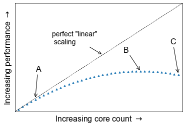
Consider the following scalability plot for a random application

At what point would you consider to be peak performance in this example.

1. A: The point where performance gains are no longer linear
2. B: The apex of the curve
3. C: The maximum core count
4. None of the above

You may find that a scalability graph my vary if you ran the same code on a different machine. Why?

Solution

1. No, the performance is still increasing, at this point we are no longer achieving perfect scalability.
2. Yes, the performance peaks at this location, and one cannot get higher speed up with this set up.
3. No, peak performance has already been achieved, and increasing the core count will onlt reduce performance.
4. No, although you can run extra benchmarks to find the exact number of cores at which the inflection point truly lies, there is no real purpose for doing so.

Tying into the answer for #4, if you produce scalability studies on different machines, they will be different because of the different setup, hardware of the machine. You are never going to get two scalability studies which are identical, but they will agree to some point.

Scaling behaviour in computation is centred around the effective use of resources as you scale up the amount of computing resources you use. An example of “perfect” scaling would be that when we use twice as many CPUs, we get an answer in half the time. “Poor” scaling would be when the answer takes only 10% less time when we double the CPUs. “Bad” scaling may see a job take longer to complete when more nodes are provided. This example is one of strong scaling, where we have a fixed problem size and need to know how quickly we can solve it. The total workload doesn’t change as we increase our resources.

The behaviour of a code in this strong scaling setting is a function of both code design and hardware layout. “Good” strong scaling behaviour occurs when the time required for computing a solution outweighs the time taken for communication to occur. Less desirable scaling performance is observed when this balance tips and communication time outweighs compute time. The point at which this occurs varies between machines and again emphasise the need for benchmarking.

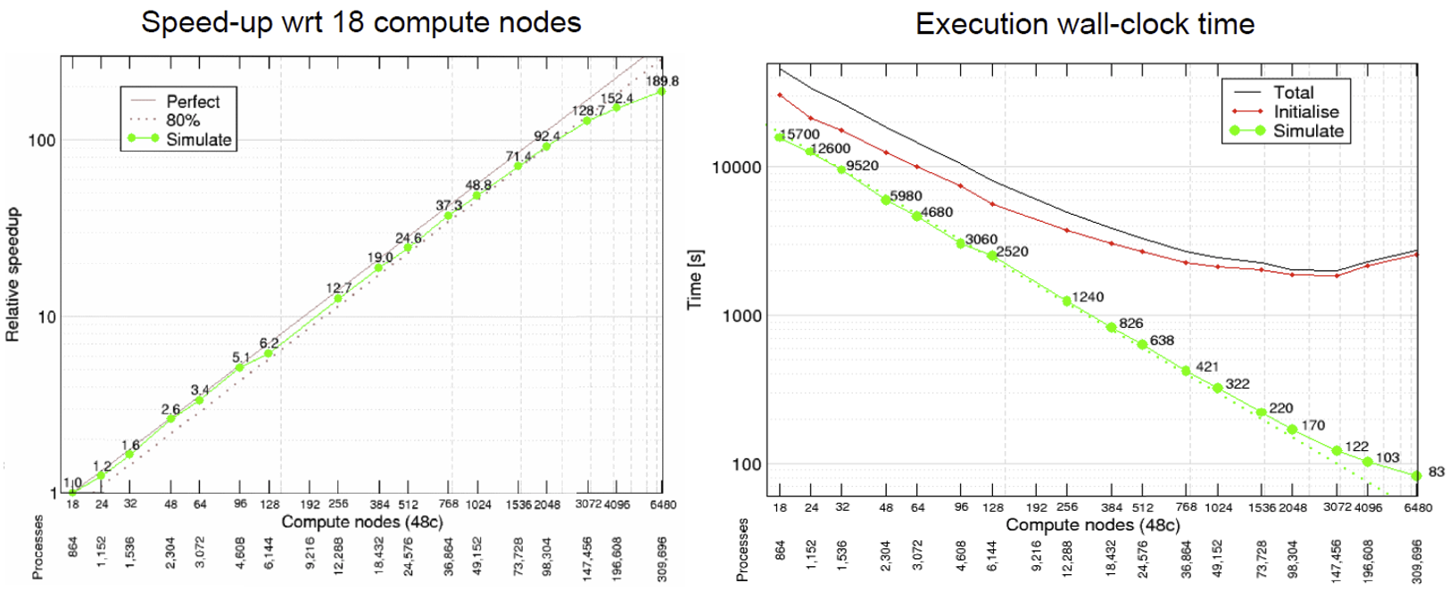
HemeLB is a code that has demonstrated very good strong scaling characteristics on several large supercomputers up to full machine scale. The plots below provide examples of such performance on the German machine SuperMUC-NG. These demonstrate how the performance varies between 864 and 309,120 CPU cores in terms of both walltime used in the simulation phase and the speed-up observed compared to the smallest number of cores used.

Plotting strong scalability

Using the original job script run HemeLB jobs at least 6 different job sizes, preferably over multiple nodes. For the size of job provided here, we suggest aiming for a maximum of around 200 cores. If your available hardware permits larger jobs, try this too up to a reasonable limit. After each job, record the Simulation Time from the Report.txt file.

Now that you have results for 2 cores, 10 cores and 2 nodes, create a scalability plot with the number of CPU cores on the X-axis and the simulation times on the Y-axis (use your favourite plotting tool, an online plotter or even pen and paper).

Are you close to “perfect” scalability?

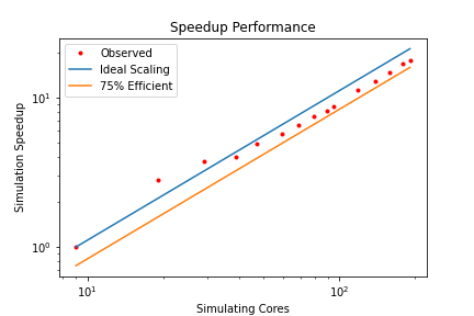
In this exercise you have plotted performance against simulation time. However this is not the only way to assess the scalability performance of the code on your machine. Speed-up is another commonly used measure. At a given core count, the speed-up can be computed by

Speedup = SimTimeAtLeastCores/SimTimeAtCurrentCores

For a perfectly scaling code, the computational speed up will match the scale-up in cores used. This line can be used as an ‘Ideal’ measure to assess local machine performance. It can also be useful to construct a line of ‘Good’ scaling - 75% efficient for example - to further assist in performance evaluation.

Some measure of algorithmic speed can also be useful for evaluating machine performance. For lattice Boltzmann method based codes such as HemeLB, a common metric is MLUPS - Millions of Lattice site Updates Per Second, which is often expressed as a core based value and can be computed by:

MLUPS = (NumSites * NumSimulationSteps)/(1e6 * SimulationTime * Cores)

When plotted over a number of simulation size for a given machine, this metric will display a steady plateau in the regime where communication is masked by computation. When this declines, it illustrates when communication begins to take much longer to perform. The point at which this occurs will depend on the size of the geometry used and the performance characteristics of the given machine. As an illustration we have generated examples of these plots for the test bifurcation case on SuperMUC-NG. We have also illustrated the effect of different axes scaling can have on presenting scaling performance. The use of logarithmic scales can allow scaling to be easily viewed but it can also make changes in values harder to assess. Linear scales make axes easier to interpret but can also make it harder to distinguish between individual points.

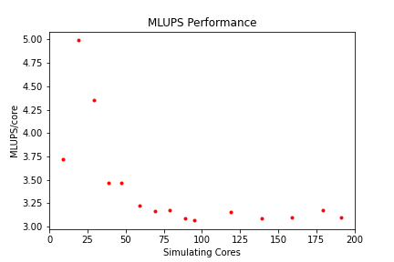
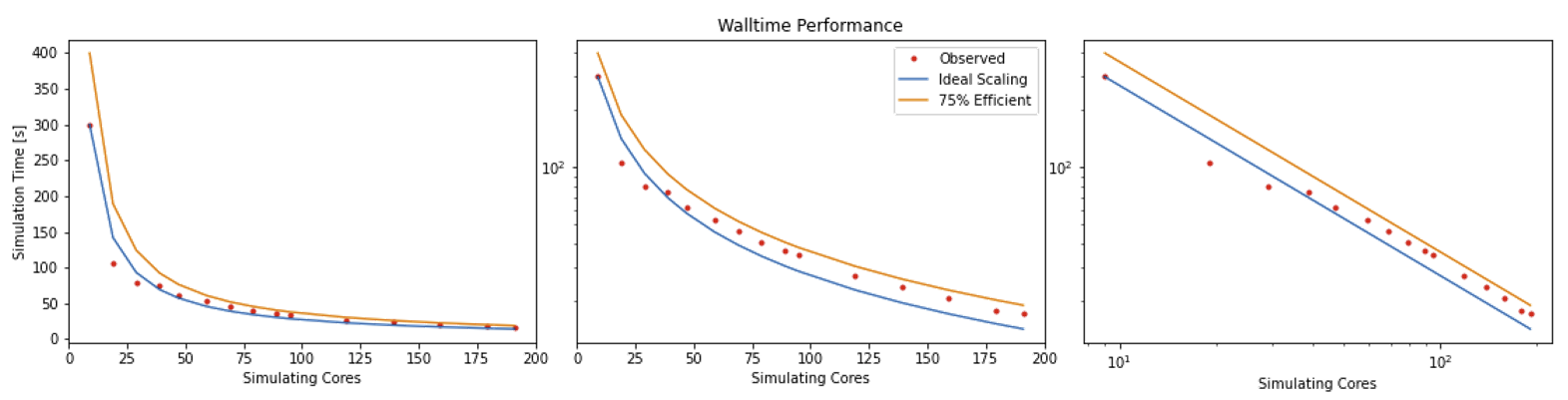
These figures also highlight two other characteristics of assessing performance. In results obtained using SuperMUC-NG, the four data points at the lowest core counts appear to have better performance than that at higher core counts. Here this is due to the the transition from one to multiple nodes on this machine and this has a consequence on communication performance. Similarly is the presence of some seemingly unusual data results. The performance of computer hardware can be occasionally variable and a single non-performant core will impact the result of the whole simulation. This emphasises the need to repeat key benchmark tests to ensure a reliable measure of performance is obtained.

Weak scaling

For weak scaling, we want usually want to increase our workload without increasing our walltime, and we do that by using additional resources. To consider this in more detail, let’s head back to our chefs again from the first episode, where we had more people to serve but the same amount of time to do it in.

We hired extra chefs who have specialisations but let us assume that they are all bound by secrecy, and are not allowed to reveal to you what their craft is, pastry, meat, fish, soup, etc. You have to find out what their specialities are, what do you do? Do a test run and assign a chef to each course. Having a worker set to each task is all well and good, but there are certain combinations which work and some which do not, you might get away with your starter chef preparing a fish course, or your lamb chef switching to cook beef and vice versa, but you wouldn’t put your pastry chef in charge of the main meat dish, you leave that to someone more qualified and better suited to the job.

Scaling in computing works in a similar way, thankfully not to that level of detail where one specific core is suited to one specific task, but finding the best combination is important and can hugely impact your code’s performance. As ever with enhancing performance, you may have the resources, but the effective use of the resources is where the challenge lies. Having each chef cooking their specialised dishes would be good weak scaling: an effective use of your additional resources. Poor weak scaling will likely result from having your pastry chef doing the main dish.

Weak scaling with HemeLB can be challenging to undertake as it is difficult to reliably guarantee an even division of work between processors for a given problem. This is due to the load partitioning algorithm used which must be able to deal with sparse and complex geometry shapes.

Key Points

• Benchmarking is a way of assessing the performance of a program or set of programs

• Strong scaling indicates how the quickly a problem of fixed size can be solved with differing number of cores on a given machine