Bottlenecks in HemeLB
Overview
Teaching: 40 min
Exercises: 45 minQuestions
How can I identify the main bottlenecks in HemeLB?
How do I come up with a strategy for minimising the impact of bottlenecks on my simulation?
What is load balancing?
Objectives
Learn how to analyse timing data in HemeLB and determine bottlenecks
Learn how to use HemeLB compilation options to overcome bottlenecks
Learn how to modify HemeLB file writing options to minimise I/O bottlenecks
Learn how the choice of simulation parameters can impact the simulation time needed to reach a solution with HemeLB
How is HemeLB parallelised?
Before using accelerator packages or other optimisation strategies to speedup your runs, it is always wise to identify what are known as performance bottlenecks. The term “bottleneck” refers to specific parts of an application that are unable to keep pace with the rest of the calculation, thus slowing overall performance. Finding these can prove dfficult at times and it may turn out that only minor tweaks are needed to speed up your code significantly.
Therefore, you need to ask yourself these questions:
- Are my simulation runs slower than expected?
- What is it that is hindering us getting the expected scaling behaviour?
HemeLB distributes communicates between the multiple CPU cores taking part in a simulation through the use of MPI. One core acts as a ‘master thread’ that coordinates the simulation whilst the remaining ‘workers’ are dedicated to solving the flow through their assigned sub-domains. It is important to note that the ‘threads’ in this case are not the same as OpenMP and used as a terminology. This work pattern can generate features of a simulation that could give rise to bottlenecks in performance. Other bottlenecks may arise from one’s choice in simulation parameters whilst others may be caused by the hardware on which a job is run.
In this episode, we will discuss some bottlenecks that may be observed within the use of HemeLB.
Identify bottlenecks
Identifying (and addressing) performance bottlenecks is important as this could save you a lot of computation time and resources. The best way to do this is to start with a reasonably representative system having a modest system size and run for a few hundred/thousand timesteps, small enough so that it doesn’t run for too long, but large enough and representative enough that you can project a full workflow.
Benchmark plots - particularly for speed-up and MLUPS/core - can help identify when a potential
bottleneck becomes a problem for efficient simulation. If an apparent bottleneck is particularly
significant, timing data from a job can also be useful in identifying where the source of it
may be. HemeLB has a reporting mechanism that we introduced in the
previous episode that provides such
information. This file gets written to results/report.txt. This file provides a wealth of information about
the simulation you have conducted, including the size of simulation conducted and the time spent in various sections
of the simulation.
We will discuss three common bottlenecks that may be encountered with HemeLB:
- Load balance
- Writing data
- Choice of parameters
In some circumstances, the options available to overcome the bottleneck may be limited. But they will provide insight into why the code is performing as observed, and can also help to ensure that accurate results are obtained.
Load balancing
One important issue with MPI-based parallelization is that it can under-perform for systems with inhomogeneous distribution of work between cores. It is pretty common that the evolution of simulated systems over time begin to reflect such a case. This results in load imbalance. While some of the processors are assigned with a finite number of lattice sites to deal with for such systems, a few processors could have far fewer sites to update. The progression of the simulation is held up by the core with the most work to do and this results in an overall loss in parallel efficiency if a large imbalance is present. This situation is more likely to expose itself as you scale up to a large large number of processors for a fixed number of sites to study.
Quantifying load imbalance
A store has 4 people working in it and each has been tasked with loading a number of boxes. Assume that each person fills a box every minute.
Person James Holly Sarah Mark Total number of boxes Number of boxes 6 1 3 2 12
- How long would it take to finish packing the boxes?
- If the work is evenly distributed among the 4 people how long would it take to fill up the boxes?
Solution
- It would take 6 minutes as James has the most number of boxes to fill. This means that Holly will have been watching for 5 minutes, Sarah for 3 and Mark for 2.
- If the work was distributed evenly, (# boxes/# people), then it would take 3 minutes to complete. Load balancing works in such a way that if a core is underutilised, it takes some work away from other ones to complete the task more quickly. This is particularly useful in chemistry/biological systems where a large area is left with little to do.
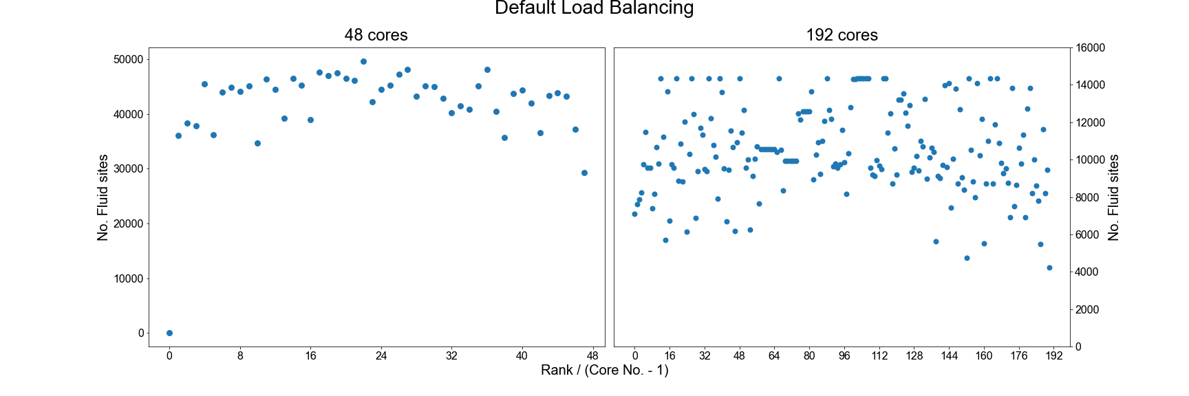
In the HemeLB results file, the number of sites assigned to each core is reported near the top of the file and can be used to check for signs of significant imbalance between cores. For example we plot below how HemeLB has distributed the workload of the bifurcation geometry on 48 and 192 cores. Note in both cases that rank 0 has no sites assigned to it. As the speed of a simulation is governed by the core with the most work to do, we do not want to see a rank that has significantly more sites than the others. Cores with significantly less workload should not hold up a simulation’s progression but will be waiting for other cores to complete and thus wasting its computational performance potential. The success of a distribution will depend on the number of cores requested and the complexity of the domain.
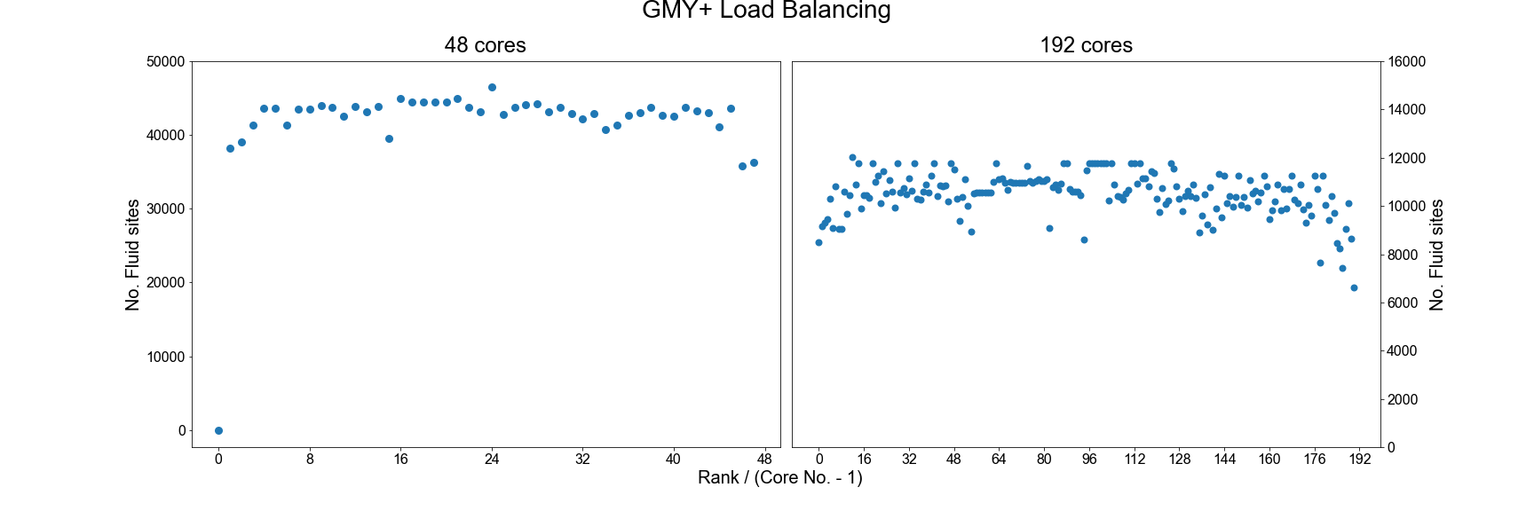
In general, the default load distribution algorithm in HemeLB has demonstrated good performance except in extreme
circumstances. This default algorithm however does assume that each node type: Bulk fluid, Inlet, Outlet, Wall;
all require the same amount of computational work to conduct and this can generate imbalance, particularly when there
are a large number of non-bulk sites present in a geometry. HemeLB has a tool available to help correct this imbalance
by assigning weights to the different site types in order to generate a more even distribution, this converts the
geometry data format from *.gmy to *.gmy+.
Compiling and using gmy2gmy+
Download the code for the gmy2gmy+ converter from
files/gmy2gmy+along with its corresponding Makefile and compile it on your machine. This script is run with the following instruction (whereDOMAINis your test domain name, eg. bifurcation.gmy):./gmy2gmy+ DOMAIN.gmy DOMAIN.gmy+ 1 2 4 4 4 4This assigns a simple weighting factor of 1 to fluid nodes, 2 to wall nodes and 4 to variants of in/outlets (in order:
Inlet,Outlet,Inlet+Wall,Outlet+Wall).Recompile HemeLB so that it knows to read
gmy+files. To keep your old executable, rename thebuildfolder tobuild_DEFAULT, so you can have abuildGMYPLUSdirectory for two executables. Edit the build script inbuildGMYPLUSto change the flag fromOFFto;-DHEMELB_USE_GMYPLUS=ONUse the tool to convert
bifurcation.gmyinto the newgmy+format.
An example of the improved load balance using the gmy+ format are shown below:
Testing the performance of gmy+
Repeat the benchmarking tests conducted in the previous episode using the
gmy+format. Rename theresultsfolder previously created to a folder name of your choice to keep your old results. You will also need to edit theinput.xmlfile accordingly) and compare your results. Also examine how load distribution has changed as a result in thereport.txtfile.Try different choices of the weights to see how this impacts your results.
Using the ParMETIS library
Another option for improving the load balance of HemeLB is to make use of the ParMETIS library that was built
as a dependency in the initial compilation of the code. To do this you will need to recompile the source code
with the following option enabled: -DHEMELB_USE_PARMETIS=ON. This tool takes the load decomposition generated
by the default HemeLB algorithm and then seeks to generate an improved decomposition.
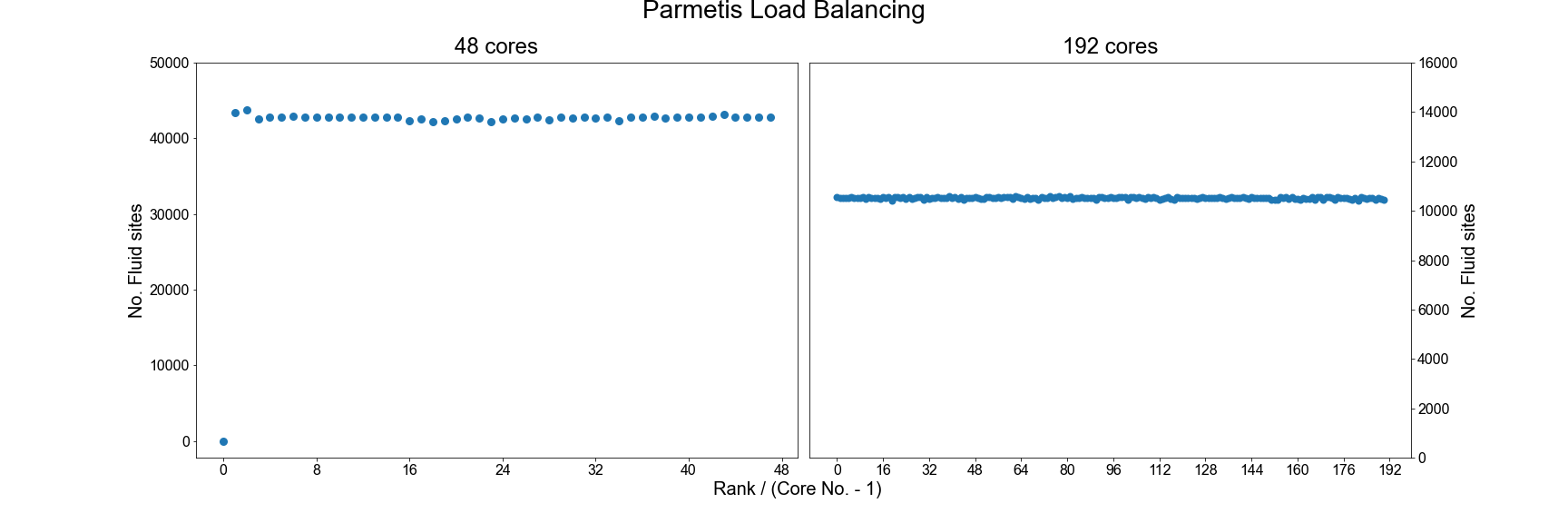
As can be seen, using ParMETIS can generate a near perfect load distribution. Whilst this may seem like an ideal solution it does come with potential drawbacks.
- Memory Usage: Some researchers have noted that ParMETIS can demand a large amount of memory during its operation and this can become a limiting factor on its use as domains become larger.
- Performance Improvement: With any of the suggested options for improving load balance, it is important to assess how much performance gain has been achieved through this change. This should be assessed in two metrics: 1) Simulation Time: This looks at the time taken for the requested iterations to complete and is the value used for assessing scaling previously. 2) Total Walltime: Includes both the Simulation Time and the time needed to initialise the simulation. The use of extra load balancing tools requires the extra initialisation time and it needs to be judged whether this extra cost is merited in terms of the achieved improvement in Simulation Time.
As many HPC systems charge for the Total Walltime of a job, it is inefficient to use a tool that causes this measure to increase. For small geometries, the initialisation time of HemeLB can be very quick (a few seconds) but for larger domains with multiple boundaries, this can extend to tens of minutes.
Testing the performance of gmy+ and ParMETIS
Repeat the benchmarking tests conducted in the previous episode using the gmy+ and ParMETIS. Once again, rename the
resultsfolder so you can keep the original and gmy+ simualtion results. Similarly, edit theinput.xmlfile so that it is looking for the gmy+ file when testing this, save as a separate file; when testing ParMETIS the originalinput.xmlfile can be used and compare your results.You should also spend some time examining how load distribution has changed as a result in the
report.txtfile.Try different choices of the gmy+ weights to see how this impacts your results. See how your results vary when a larger geometry is used (see
files/biggerBifforgmyand input files).Example Results
Note that exact timings can vary between jobs, even on the same machine - you may see different performances. The relative benefit of using load balancing schemes will vary depending on the size and complexity of the domain, the length of your simulation and the available hardware.
Scheme Cores Initialisation Time (s) Simulation Time (s) Total Time (s) Default 48 0.7 56.0 56.7 Default 192 1.0 15.3 16.3 GMY+ 48 0.7 56.1 56.8 GMY+ 192 1.0 13.2 14.2 ParMETIS 48 2.6 56.7 59.3 ParMETIS 192 2.4 12.5 14.9
Data writing
With all simulations, it is important to get output data to assess how the simulation has performed and to investigate your problem of interest. Unfortunately, writing data to disk is a cost that can negatively impact on simulation performance. In HemeLB, output is governed by the ‘properties’ section of the input file.
 <properties>
    <propertyoutput file="whole.dat" period="1000">
      <geometry type="whole" />
      <field type="velocity" />
      <field type="pressure" />
    </propertyoutput>
    <propertyoutput file="inlet.dat" period="100">
      <geometry type="inlet" />
      <field type="velocity" />
      <field type="pressure" />
    </propertyoutput>
    <propertyoutput file="outlet.dat" period="100">
      <geometry type="inlet" />
      <field type="velocity" />
      <field type="pressure" />
    </propertyoutput>
  </properties>
</hemelbsettings>
In this example, we output pressure and velocity information at the inlet and outlet surfaces of our domain every 100
steps and for the whole simulation domain every 1000 steps. This data is written to compressed *.dat files in
results/Extracted. It is recommended that the whole option is used with caution as it can generate VERY large
*.dat files. The larger your simulation domain, the greater the effect of data writing will be.
Testing the effect of data writing
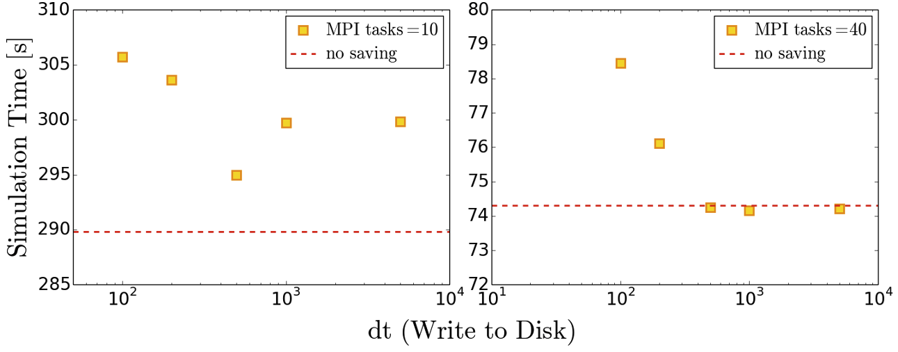
Repeat the benchmarking tests conducted in the previous episode now outputting inlet/outlet and whole data at a number of different time intervals. Compare your results to those you have previously obtained. Given output is critical to the simulation process what would be a suitable strategy for writing output data?
Below we provide some example results obtained on SuperMUC-NG by writing the whole data set at different time intervals. The impact on performance is clear to observe.
Effect of model size
In
files/biggerBifyou can find a higher resolution model ( ≈ 4 times larger) of the bifurcation model we have been studying. Repeat some of the exercises on load balancing and data writing to see how a larger model impacts the performance of your system.
Choice of simulation parameters
With most simulation methods, results that accurately represent the physical system being studied can only be achieved if suitable parameters are provided. When this is not the case, the simulation may be unstable, it may not represent reality or both. Whilst the choice of simulation parameters may not change the algorithmic speed of your code, they can impact how long a simulation needs to run to represent a given amount of physical time. The lattice Boltzmann method, on which HemeLB is based, has specific restrictions that link the discretization parameters, physical variables and simulation accuracy and stability.
In these studies, HemeLB is using a single relaxation time (or BGK) collision kernel to solve the fluid flow. HemeLB (and the lattice Boltzmann method more widely) also has other collision kernels that can permit simulation of more sophisticated flow scenarios such as non-Newtonian fluid rheology or possess improved stability or accuracy characteristics. The BGK kernel is typically the first choice for the collision model to used and is also simplest (and generally fastest) to implement and perform computationally. In this model viscosity, lattice spacing, and simulation timestep are related to the relaxation parameter τ by,
ν = 1/3(τ - ½) Δx2/Δt
Here:
- ν - Fluid viscosity [m2/s] - in HemeLB this is set to 4x10⁻⁶ m2/s the value for human blood
- Δx - Lattice spacing [m]
- Δt - Time step [s]
This relationship puts physical and practical limits on the values that can be selected for these parameters. In particular, τ > ½ must be imposed for a physical viscosity to exist, values of τ very close to ½ can be unstable. Generally, a value of τ ≈ 1 gives the most accurate results.
The lattice Boltzmann method can only replicate the Navier-Stokes equations for fluid flow in a low Mach number regime. In practice, this means that the maximum velocity of the simulation must be significantly less than the speed of sound of the simulation. As a rough rule of thumb, the following is often acceptable in simulations (though if smaller Ma can be achieved, this is better):
Ma = (3umax*Δt)⁄Δx
Often the competing restrictions placed on a simulation by these two expressions can demand a small time step to be used.
Determining your physical parameters
Suppose you wish to simulate blood flow through a section of the aorta with a maximum velocity of 1 m/s for a period of two heartbeats (2 seconds). Using the expressions above, determine suitable choices for the time step if your geometry has a grid resolution of Δx = 100 μm.
How many iterations do you need to run for this choice? How do your answers change if you have higher resolutions models with (i) Δx = 50 μm and (ii) Δx = 20 μm? What would be the pros and cons of using these higher resolution models?
Solution
Starting points would be the following, these would likely need further adjustment in reality:
- For Δx = 100 μs, Δt = 5 μs gives Ma ≈ 0.087 and τ = 0.506; 400,000 simulation steps required
- For Δx = 50 μs, Δt = 2.5 μs gives Ma ≈ 0.087 and τ = 0.512; 800,000 simulation steps required
- For Δx = 20 μs, Δt = 1 μs gives Ma ≈ 0.087 and τ = 0.530; 2,000,000 simulation steps required
Higher resolution geometries have many more data points stored within them - halving the grid resolution requires approximately 8x more points and will take roughly 16x longer to simulate for the same Ma and physical simulation time. Higher resolution domains also generate larger data output, which can be more challenging to analyse. The output generated should also be a more accurate representation of the reality being simulated and can achieve more stable simulation parameters.
Key Points
The best way to identify bottlenecks is to run different benchmarks on a smaller system and compare it to a representative system
Effective load balancing is being able to distribute an equal amount of work across processes.
Evaluate both simulation time and overall wall time to determine if improved load balance leads to more efficient performance.
The choice of simulation parameters impacts both the accuracy and stability of a simulation as well as the time needed to complete a simulation. This is especially true for solvers using explicit techniques such as HemeLB.
For all applications, writing data to file can be a time consuming activity. Carefully consider what data you need for post-processing to minimise the time spent in this regime.