Why bother with performance?

Overview

Teaching: 10 min
Exercises: 5 min

Questions

• What is software performance?

• Why is software performance important?

• How can performance be measured?

• What is meant by flops, walltime and CPU hours?

• How can performance be enhanced?

• How can I use compute resources effectively?

Objectives

• Understand the link between software performance and hardware

• Identify the different methods of enhancing performance

• Calculate walltime, CPU hours

What is software performance?

The concept of performance is generic and can apply to many factors in our lives, such as our own physical and mental performance. With software performance the emphasis is not on using the most powerful machine, but on how best to utilise the power that you have.

Imagine you are the chef in a restaurant and you are able to prepare the perfect dish, every time You are also able to produce a set 7 course meal for a table of 3-6 without too much difficulty. If you are catering a conference dinner though, it becomes more difficult, as people would be waiting many hours for their food. However, if you could delegate tasks to a team of 6 additional chefs who could assist you (while also communicating with each other), you have a much higher chance of getting the food out on time and coping with a large workload. With 7 courses and a total of 7 chefs, it’s most likely that each chef will spend most of their time concentrating on doing one course.

When we dramatically increase the workload we need to distribute it efficiently over the resources we have available so that we can get the desired result in a reasonable amount of time. That is the essence of software performance, using the resources you have to the best of their capabilities.

Why is software performance important?

This is potentially a complex question but has a pretty simple answer when we restrict ourselves to the context of this lesson. Since the focus here is our usage of software that is developed by someone else, we can take a self-centred and simplistic approach: all we care about is reducing the time to solution to an acceptable level while minimising our resource usage.

This lesson is about taking a well-informed, systematic approach towards how to do this.

Enhancing performance: rationale

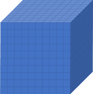
Imagine you had a 10x10x10 box like the one below, divided up into smaller boxes, each measuring 1x1x1. In one hour, one CPU core can simulate one hour of activity inside the smaller box. If you wanted to simulate what was happening inside the large box for 8 hours, how long will it take to run if we only use one CPU core?

Solution

8000 hours…close to a year!

This is way longer than is feasibly convenient! But remember, that is utilising just one core. If you had a machine that could simulate each of those smaller boxes simultaneously and a code that enables each box to effectively interact with each other, the whole job would only take roughly an hour (but probably a little more because of issues we will discuss in subsequent episodes).

How is performance measured?

There are a number of key terms in computing when it comes to understanding performance and expected duration of tasks. The most important of these are walltime, flops and CPU hours.

Walltime

Walltime is the length of time, usually measured in seconds, that a program takes to run (i.e., to execute its assigned tasks). It is not directly related to the resources used, it’s the time it takes according to an independent clock on the wall.

Flops

Flops (or sometimes flop/s) stands for floating point operations per second and they are typically used to measure the (theoretical) performance of a computer’s processor.

The theoretical peak flops is given by

Number of cores * Average frequency * Operations per cycle

What a software program can achieve in terms of flops is usually a surprisingly small percentage of this value (e.g., 10% efficiency is not a bad number!).

Since in our case we don’t develop or compile the code, the only influence we have on the flops achieved by the application is by dictating the choices it makes during execution (sometimes called telling it what code path to walk).

CPU Hours

CPU hours is the amount of CPU time spent processing. For example, if I execute for a walltime of 1 hour on 10 CPUs, then I will have used up 10 CPU hours.

Maximising the flops of our application will help reduce the CPU hours, since we will squeeze more calculations out of the same CPU time. However, you can achieve much greater influence on the CPU hours by using a better algorithm to get to your result. The best algorithm choice is usually heavily dependent on your particular use case (and you are always limited by what algorithm options are available in the software).

Calculate CPU hours

Assume that you are utilising all the available cores in a node with 40 CPU cores. Calculate the CPU hours you would need if you expect to run for 5 hours using 2 nodes.

How much walltime do you need?

How do you ask the resource scheduler for that much time?

Solution

400 CPU hours are needed.

We need to ask the scheduler for 5 hours (and 2 nodes worth of resources for that time). To ask for this from the scheduler we need to include the appropriate option in our job script:

#SBATCH --time 5:00:00

The --time option to the scheduler used in the exercise indicates the maximum amount of walltime requested, which will differ from the actual walltime the code spends to run. It is important to overestimate this number so that it doesn’t kill your job before it has finished running.

How can we enhance performance?

If you are taking this course you are probably application users, not application developers. To enhance the code performance you need to trigger behaviour in the software that the developers will have put in place to potentially improve performance. To do that, you need to know what the triggers are and then try them out with your use case to see if they really do improve performance.

Some triggers will be hardware related, like the use of OpenMP, MPI, or GPUs. Others might relate to alternative libraries or algorithms that could be used by the application.

Enhancing Performance

Which of these are viable ways of enhancing performance? There may be more than one correct answer.

1. Utilising more CPU cores and nodes
2. Increasing the simulation walltime
3. Reduce the frequency of file writing in the code
4. Having a computer with higher flops

Solution

1. Yes, potentially, the more cores and nodes you have, the more work can be distributed across those cores… but you need to ensure they are being used!
2. No, increasing simulation walltime only increases the possible duration the code will run for. It does not improve the code performance.
3. Yes, IO is a very common bottleneck in software, it can be very expensive (in terms of time) to write files. Reducing the frequency of file writing can have a surprisingly large impact.

4. Yes, in a lot of cases the faster the computer, the faster the code can run. However, you may not be able to find a computer with higher flops, since higher individual CPU flops need disproportionately more power to run (so are not well suited to an HPC system).

   In an HPC system, you will usually find a lot of lower flop cores because they make sense in terms of the use of electrical energy. This surprises people because when they move to an HPC system, they may initially find that their code is slower rather than faster. However, this is usually not about the resources but managing their understanding and expectations of them.

As you can see, there are a lot of right answers, however some methods work better than others, and it can entirely depend on the problem you are trying to solve.

How can I use compute resources effectively?

Unfortunately there is no simple answer to this, because the art of getting the ‘optimum’ performance is ambiguous. There is no ‘one size fits all’ method to performance optimization.

While preparing for production use of software, it is considered good practice to test performance on manageable portion of your problem first, attempt to optimize it (using some of the recommendations we outline in this lesson, for example) and then make a decision about how to run things in production.

Key Points

• Software performance is the use of computational resources effectively to reduce runtime

• Understanding performance is the best way of utilising your HPC resources efficiently

• Performance can be measured by looking at flops, walltime, and CPU hours

• There are many ways of enhancing performance, and there is no single ‘correct’ way. The performance of any software will vary depending on the tasks you want it to undertake.

Connecting performance to hardware

Overview

Teaching: 15 min
Exercises: 5 min

Questions

• How can I use the hardware I have access to?

• What is the difference between OpenMP and MPI?

• How can I use GPUs and/or multiple nodes?

Objectives

• Differentiate between OpenMP and MPI

Accelerating performance

To speed up a calculation in a computer you can either use a faster processor or use multiple processors to do parallel processing. Increasing clock-speed indefinitely is not possible, so the best option is to explore parallel computing. Conceptually this is simple: split the computational task across different processors and run them all at once, hence you get the speed-up.

In practice, however, this involves many complications. Consider the case when you are having just a single CPU core, associated RAM (primary memory: faster access of data), hard disk (secondary memory: slower access of data), input (keyboard, mouse) and output devices (screen).

Now consider you have two or more CPU cores, you would notice that there are many things that you suddenly need to take care of:

1. If there are two cores there are two possibilities: Either these two cores share the same RAM (shared memory) or each of these cores have their own RAM (private memory).
2. In case these two cores share the same RAM and write to the same place at once, what would happen? This will create a race condition and the programmer needs to be very careful to avoid such situations!
3. How to divide and distribute the jobs among these two cores?
4. How will they communicate with each other?
5. After the job is done where the final result will be saved? Is this the storage of core 1 or core 2? Or, will it be a central storage accessible to both? Which one prints things to the screen?

Shared memory vs Distributed memory

When a system has a central memory and each CPU core has a access to this memory space it is known as a shared memory platform. However, when you partition the available memory and assign each partition as a private memory space to CPU cores, then we call this a distributed memory platform. A simple graphic for this is shown below:

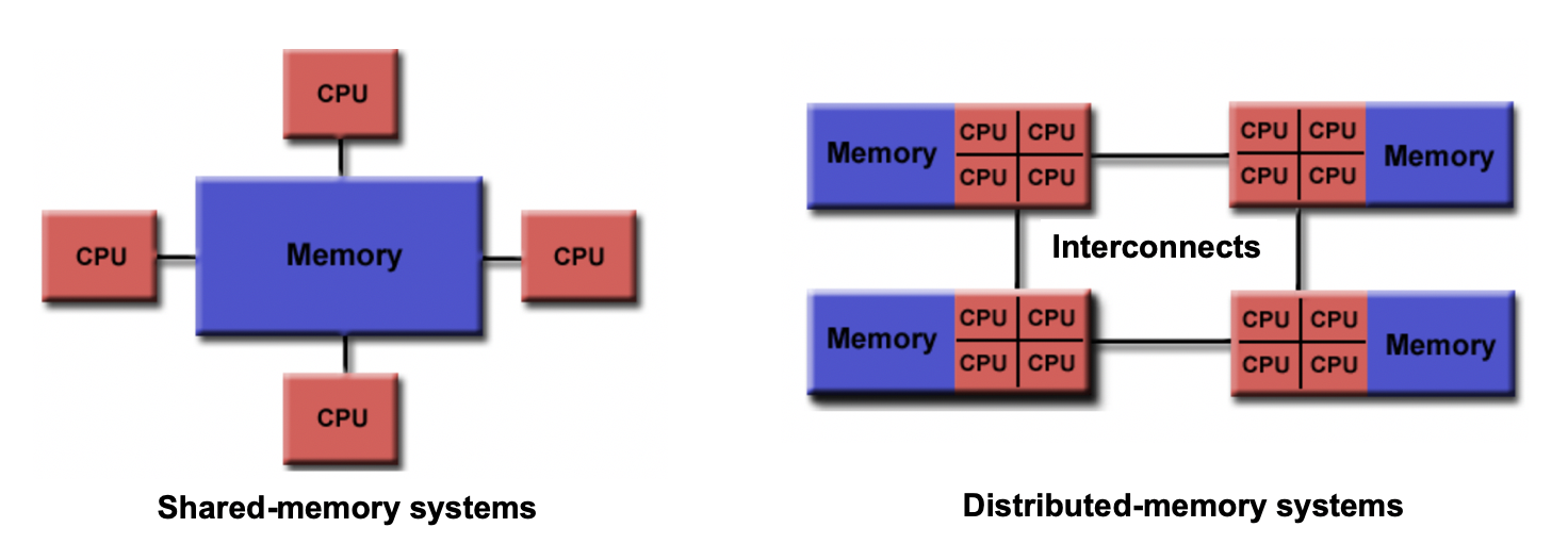
Depending upon what kind of memory a computer has, the parallelization approach of a code could vary. For example, in a distributed memory platform, when a CPU core needs data from its private memory, it is fast to get it. But, if it requires access to a data that resides in the private memory of another CPU core then it requires a ‘communication’ protocol and data access becomes slower.

Similar situation arises for GPU coding too. In this case, the CPU is generally called the host and the GPUs are called the device. When we submit a GPU job, it is launched in the CPU (host) which in turn directs it to be executed by the GPUs (devices). While doing these calculations, data is copied from CPU memory to the GPU’s and then processed. After the GPU finishes a calculation, the result is copied back from the GPU to CPU. This communication is expensive and it could significantly slow down a calculation if care is not taken to minimize it. We’ll see later in this tutorial that communication is a major bottleneck in many calculations and we need to devise strategies to reduce the related overhead.

In shared memory platforms, the memory is being shared by all the processors. In this case, the processors communicate with each other directly through the shared memory…but we need to take care that the access the memory in the right order!

Parallelizing an application

When we say that we parallelize an application, we actually mean we devise a strategy that divides the whole job into pieces and assign each piece to a worker (CPU core or GPU) to help solve. This parallelization strategy depends heavily on the memory structure. For example, if we want to use OpenMP, it provides a thread level parallelism that is well-suited for a shared memory platform, but you can not use it in a distributed memory system. For a distributed memory system, you need a way to communicate between workers (a message passing protocol), like MPI.

Multithreading

If we think of a process as an instance of your application, multithreading is a shared memory parallelization approach which allows a single process to contain multiple threads which share the process’s resources but work relatively independently. OpenMP and CUDA are two very popular multithreading execution models that you may have heard of. OpenMP is generally used for multi-core/many-core CPUs and CUDA is used to utilize threading for GPUs.

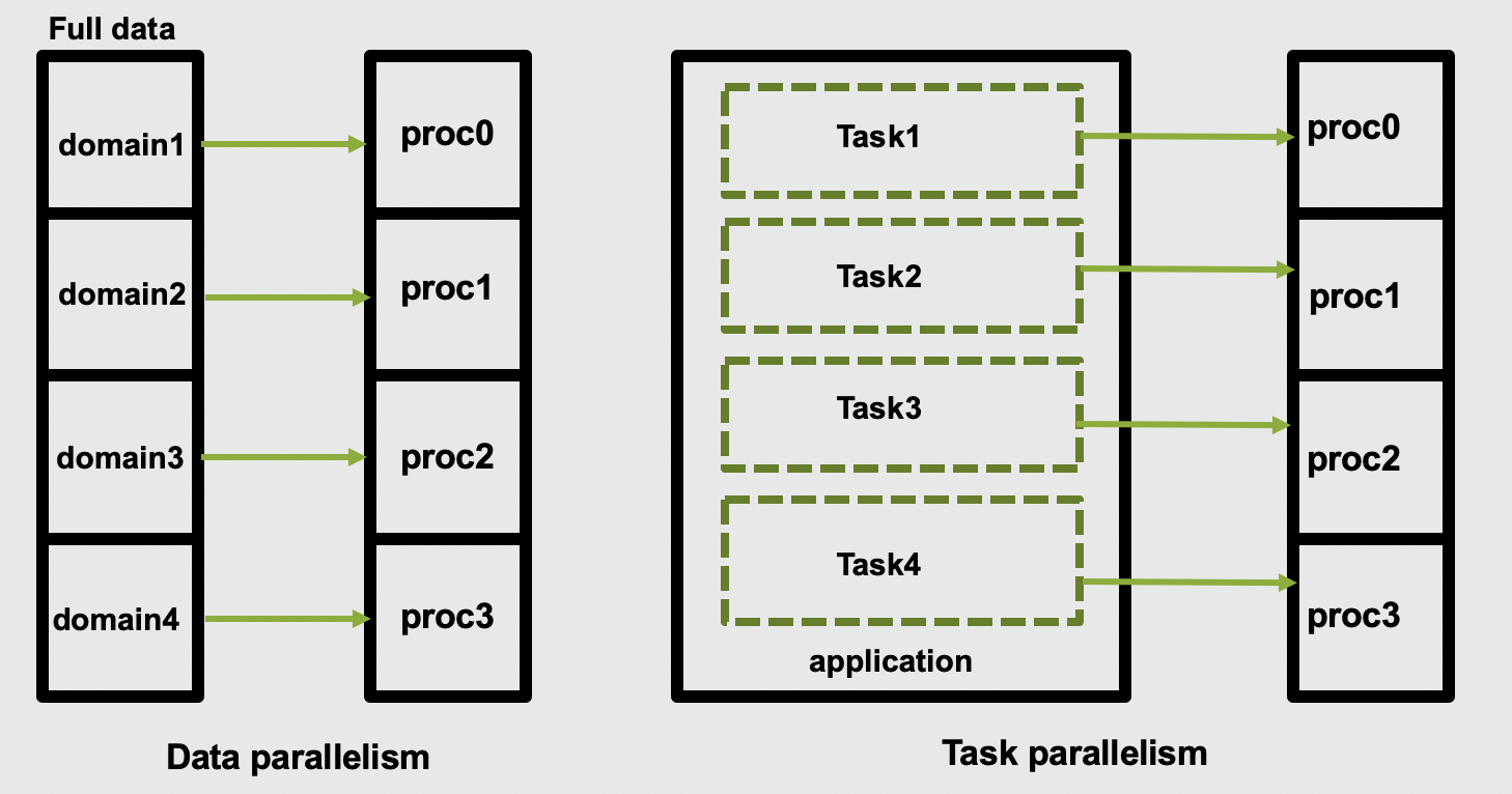
The two main parallelization strategies are data parallelism and task parallelism. In data parallelism, some set of tasks are performed by each core using different subsets of the same data. Task parallelism is when we can decompose the larger task into multiple independent sub-tasks, each of which we then assign to different cores. A simple graphical representation is given below:

As application users, we need to know if our application actually offers control over which parallelization methods (and tools) we can use. If so, we then need to figure out how to make the right choices based on our use case and the hardware we have available to us.

Popular parallelization strategies

The main parallelisation technique that is used by any modern software is the domain decomposition method. In this process, the global domain is divided into many sub-domains and then each sub-domain is assigned to a processor. If your computer has N physical processors, you can initiate N MPI processes on your computer. This means each sub-domain is handled by a MPI process and when atoms move from one domain to another, the atom identities assigned to each MPI task will also be updated accordingly. In this method, for a (nearly) homogeneously distributed atomic system, we can expect almost uniform distribution of work across various MPI tasks.

What is MPI?

A long time before we had smart phones, tablets or laptops, compute clusters were already around and consisted of interconnected computers that had about enough memory to show the first two frames of a movie (2 x 1920 x 1080 x 4 Bytes = 16 MB). However, scientific problems back than were demanding more and more memory (as they are today). To overcome the lack of adequate memory, specialists from academia and industry came up with the idea to consider the memory of several interconnected compute nodes as one. They created a standardized software that synchronizes the various states of memory through the network interfaces between the client nodes during the execution of an application. With this performing large calculations that required more memory than each individual node can offer was possible.

Moreover, this technique of passing messages (hence Message Passing Interface or MPI) on memory updates in a controlled fashion allow us to write parallel programs that are capable of running on a diverse set of cluster architectures.(Reference: https://psteinb.github.io/hpc-in-a-day/bo-01-bonus-mpi-for-pi/ )

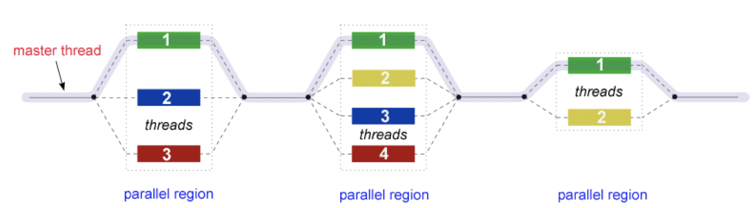
In addition to MPI, some applications also support thread level parallelism (through, for example OpenMP directives) which can offer additional parallelisation within a subdomain. The basic working principle in OpenMP is based the “Fork-Join” model, as shown below.

In the ‘Fork-Join’ model, there exists a master thread which “fork”s into multiple threads. Each of these forked-threads executes a part of the whole job and when all the threads are done with their assigned jobs, these threads join together again. Typically, the number of threads is equal to the number of available cores, but this can be influenced by the application or the user at run-time.

Using the maximum possible threads on a node may not always provide the best performance. It depends on many factors and, in some cases,the MPI parallelization strategy is so strongly integrated that it almost always offers better performance than the OpenMP based thread-level parallelism.

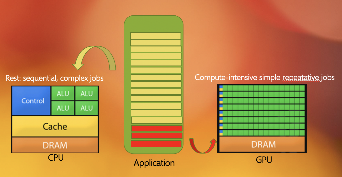
Another commonly found parallelization strategy is to use GPUs (with the more general term being an accelerator). GPUs work together with the CPUs. A CPU is specialized to perform complex tasks (like making decisions), while a GPU is very efficient in doing simple, repetitive, low level tasks. This functional difference between a GPU and CPU could be attributed to the massively parallel architecture that a GPU possesses. A modern CPU has relatively few cores which are well optimized for performing sequential serial jobs. On the contrary, a GPU has thousands of cores that are highly efficient at doing simple repetitive jobs in parallel. See below on how a CPU and GPU works together.

Using all available resources

Say you’ve actually got a powerful desktop with multiple CPU cores and a GPU at your disposal, what are good options for leveraging them?

1. Utilising MPI (Message Passing Interface)
2. Utilising OpenMP (Open Multi-Processing)
3. Using performance enhancing libraries or plugins
4. Use GPUs instead of CPUs
5. Splitting code up into smaller individual parts

Solution

1. Yes, MPI can enable you to split your code into multiple processes distributed over multiple cores (and even multiple computers), known as parallel programming. This won’t help you to use the GPU though.
2. Yes, like MPI this is also parallel programming, but deals with threads instead of processes, by splitting a process into multiple threads, each thread using a single CPU core. OpenMP can potentially also leverage the GPU.
3. Yes, that is their purpose. However, different libraries/plugins run on different architectures and with different capabilities, in this case you need something that will leverage the additional cores and/or the GPU for you.
4. Yes, GPUs are better at handling multiple simple tasks, whereas a CPU is better at running complex singular tasks quickly.
5. It depends, if you have a simulation that needs to be run from start to completion, then splitting the code into segments won’t be of any benefit and will likely waste compute resources due to the associated overhead. If some of the segments can be run simultaneously or on different hardware then you will see benefit…but it is usually very hard to balance this.

Key Points

• OpenMP works on a single node, MPI can work on multiple nodes

Benchmarking and Scaling

Overview

Teaching: 30 min
Exercises: 15 min

Questions

• What is benchmarking?

• How do I do a benchmark?

• What is scaling?

• How do I perform a scaling analysis?

Objectives

• Be able to perform a benchmark analysis of an application

• Be able to perform a scaling analysis of an application

• Understand what good scaling performance looks like

What is benchmarking?

To get an idea of what we mean by benchmarking, let’s take the example of a sprint athlete. The athlete runs a predetermined distance on a particular surface, and a time is recorded. Based on different conditions, such as how dry or wet the surface is, or what the surface is made of (grass, sand, or track) the times of the sprinter to cover a distance (100m, 200m, 400m etc) will differ. If you know where the sprinter is running, and what the conditions were like, when the sprinter sets a certain time you can cross-correlate it with the known times associated with certain surfaces (our benchmarks) to judge how well they are performing.

Benchmarking in computing works in a similar way: it is a way of assessing the performance of a program (or set of programs), and benchmark tests are designed to mimic a particular type of workload on a component or system. They can also be used to measure differing performance across different systems. Usually codes are tested on different computer architectures to see how a code performs on each one. Like our sprinter, the times of benchmarks depends on a number of things: software, hardware or the computer itself and it’s architecture.

Callout: Local vs system-wide installations

Whenever you get access to an HPC system, there are usually two ways to get access to software: either you use a system-wide installation or you install it yourself. For widely used applications, it is likely that you should be able to find a system-wide installation. In many cases using the system-wide installation is the better option since the system administrators will (hopefully) have configured the application to run optimally for that system. If you can’t easily find your application, contact user support for the system to help you.

For less widely used codes, such as HemeLB, you will have to compile the code on the HPC system for your own use. Build scripts are available to help streamline this process but these must be customised to the specific libraries and nomenclature of individual HPC systems.

In either case, you should still check the benchmark case though! Sometimes system administrators are short on time or background knowledge of applications and do not do thorough testing. For locally compiled codes, the default options for compilers and libraries may not necessarily be optimal for performance. Benchmark testing can allow the best option for that machine to be identified.

The ideal benchmarking study

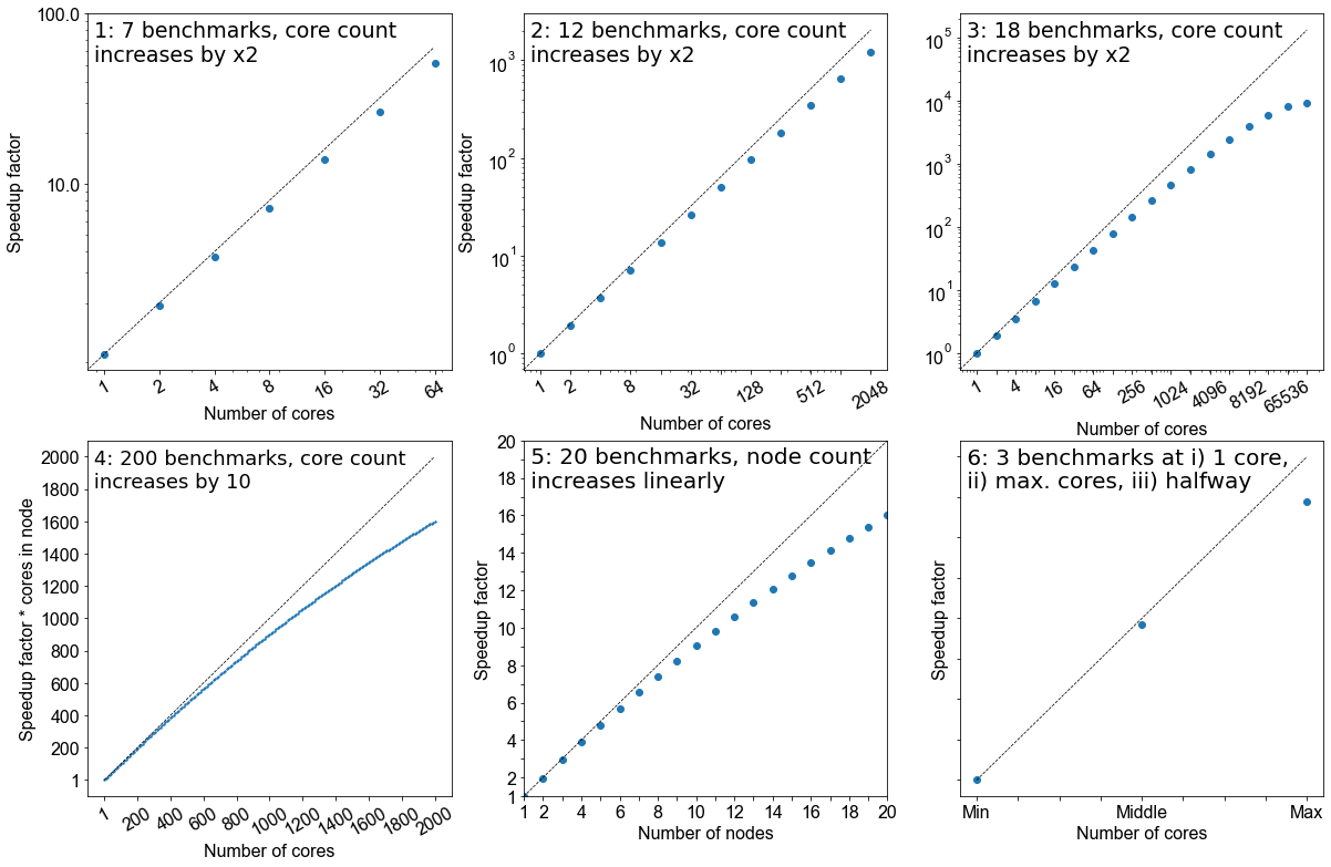
Benchmarking is a process that judges how well a piece of software runs on a system. Based on what you have learned thus far from running your own benchmarks, which of the following would represent a good benchmarking analysis?

1. 7 benchmarks, core count increases by factor of 2
2. 12 benchmarks, core count increases by factor of 2
3. 18 benchmarks, core count increases by factor of 2
4. 200 benchmarks, core count increases by 10
5. 20 benchmarks, node count increases linearly
6. 3 benchmarks; i) 1 core, ii) the maximum of cores possible, iii) a point at halfway

Solution

1. No, the core counts that are being benchmarked are too low and the number of points is not sufficient
2. Yes, but depends on the software you are working with, how you want to use it, and how big your system is. This does not give a true view how scalable it is at higher core counts.
3. Yes. If the system allows it and you have more cores at your disposal, this is the ideal benchmark to run. But as with #2, it depends on how you wish to utlise the software.
4. No, although it increases by a factor of 10 to 2000 cores, there are too many points on the graph and therefore would be highly impractical. Benchmarks are used to get an idea of scalability, the exact performance will vary with every benchmark run.
5. Yes. This is also a suitable metric for benchmarking, similar to response #3.
6. No. While this will cover the spread of simulation possibilities on the machine, it will be too sparse to permit an appropriate characterisation of the the code on your system. Depending on the operational restrictions of your system, full machine jobs may not be possible to run or may require a long time before it launches.

Creating a job file

HPC systems typically use a job scheduler to manage the deployment of jobs and their many different resource requests from multiple users. Common examples of schedulers include SLURM and PBS.

We will now work on creating a job file which we can run on SuperMUC-NG. Writing a job file from scratch is error prone, and most supercomputing centres will have a basic one which you can modify. Below is a job file we can use and modify for the rest of the course.

#!/bin/bash
# Job Name and Files
#SBATCH -J jobname

#Output and error:
#SBATCH -o ./%x.%j.out
#SBATCH -e ./%x.%j.err
#Initial working directory:
#SBATCH -D ./

# Wall clock limit:
#SBATCH --time=00:15:00

#Setup of execution environment
#SBATCH --export=NONE
#SBATCH --get-user-env
#SBATCH --account="projectID"
#SBATCH --partition="Check Local System"

#Number of nodes and MPI tasks per node:
#SBATCH --nodes=1
#SBATCH --ntasks-per-node=10

#Add 'Module load' statements here - check your local system for specific modules/names
module purge 
module load slurm_setup 
module load intel/19.0.5 
module load intel-mpi/2019-intel

#Run HemeLB 
rm -rf results #delete old results file
mpiexec -n $SLURM_NTASKS /dss/dsshome1/00/di39tav2/codes/HemePure/src/build_PP/hemepure -in input.xml -out results

Particular information includes who submitted the jobs, how long it needs to run for, what resources are required and which allocation needs to be charged for the job. After this job information, the script loads the libraries necessary for supporting jobs execution. In particular, the compiler and MPI libraries need to be loaded. Finally the commands to launch the jobs are called. These may also include any pre- or post-processing jobs that need to be run on the compute nodes.

The example above submits a HemeLB job on 1 node that utilises 10 cores and runs for a maximum of 10 minutes. Where indicated, modify the script to the correct settings for usernames and filepaths for your HPC system. It must be noted here that all HPC systems have subtle differences in the necessary commands to submit a job, you should consult your local documentation for definitive advice on this for your HPC system.

Running a HemeLB job on your HPC

Examine the provided jobscript, which is located in files/2c-bifJobScript-slurm.sh, and modify accordingly so the correct modules are loaded and the path you where the hemepure executable is correct. You can run the job using sbatch myjob.sh. You can track the progress of the job using squeue yourUsername. This job uses 2 cores and will take about 10-15 minutes.

Once you are confident that the details in the job script are correct, we will repeat this with 10 cores, so copt the job script you have been working on and move it into files/10core-bif and modify it so that it runs on 10 cores.

Do you notice a speedup?

While these job is running, lets examine the input file to understand the HemeLB job we have submitted.

<?xml version="1.0"?>
<hemelbsettings version="3">
  <simulation>
    <step_length units="s" value="1e-5"/>
    <steps units="lattice" value="5000"/>
    <stresstype value="1"/>
    <voxel_size units="m" value="5e-5"/>
    <origin units="m" value="(0.0,0.0,0.0)"/>
  </simulation>
  <geometry>
    <datafile path="bifurcation.gmy"/>
  </geometry>
  <initialconditions>
    <pressure>
      <uniform units="mmHg" value="0.000"/>
    </pressure>
  </initialconditions>
  <monitoring>
    <incompressibility/>
  </monitoring>
  <inlets>
    <inlet>
      <condition subtype="cosine" type="pressure">
        <amplitude units="mmHg" value="0.0"/>
        <mean units="mmHg" value="0.001"/>
        <phase units="rad" value="0.0"/>
        <period units="s" value="1"/>
      </condition>
      <normal units="dimensionless" value="(0.707107,-2.4708e-12,-0.707107)"/>
      <position units="lattice" value="(26.2137,35.8291,372.094)"/>
    </inlet>
  </inlets>
  <outlets>
    <outlet>
      <condition subtype="cosine" type="pressure">
        <amplitude units="mmHg" value="0.0"/>
        <mean units="mmHg" value="0.0"/>
        <phase units="rad" value="0.0"/>
        <period units="s" value="1"/>
      </condition>
      <normal units="dimensionless" value="(4.15565e-13,1.44689e-12,1)"/>
      <position units="lattice" value="(165.499,35.8291,3)"/>
    </outlet>
    <outlet>
      <condition subtype="cosine" type="pressure">
        <amplitude units="mmHg" value="0.0"/>
        <mean units="mmHg" value="0.0"/>
        <phase units="rad" value="0.0"/>
        <period units="s" value="1"/>
      </condition>
      <normal units="dimensionless" value="(-0.707107,-4.27332e-12,-0.707107)"/>
      <position units="lattice" value="(304.784,35.8291,372.094)"/>
    </outlet>
  </outlets>
  <properties>
	<propertyoutput file="whole.dat" period="100">
      <geometry type="whole" />
      <field type="velocity" />
      <field type="pressure" />
    </propertyoutput>
    <propertyoutput file="inlet.dat" period="100">
      <geometry type="inlet" />
      <field type="velocity" />
      <field type="pressure" />
  </propertyoutput>
</properties>
</hemelbsettings>

The HemeLB input file can be broken into three main regions:

1. Simulation set-up: specify global simulation information like discretisation parameters, total simulation steps and initialisation requirements
2. Boundary conditions: specify the local parameters needed for the execution of the inlets and outlets of the simulation domain
3. Property output: dictates the type and frequency of dumping simulation data to file for post-processing

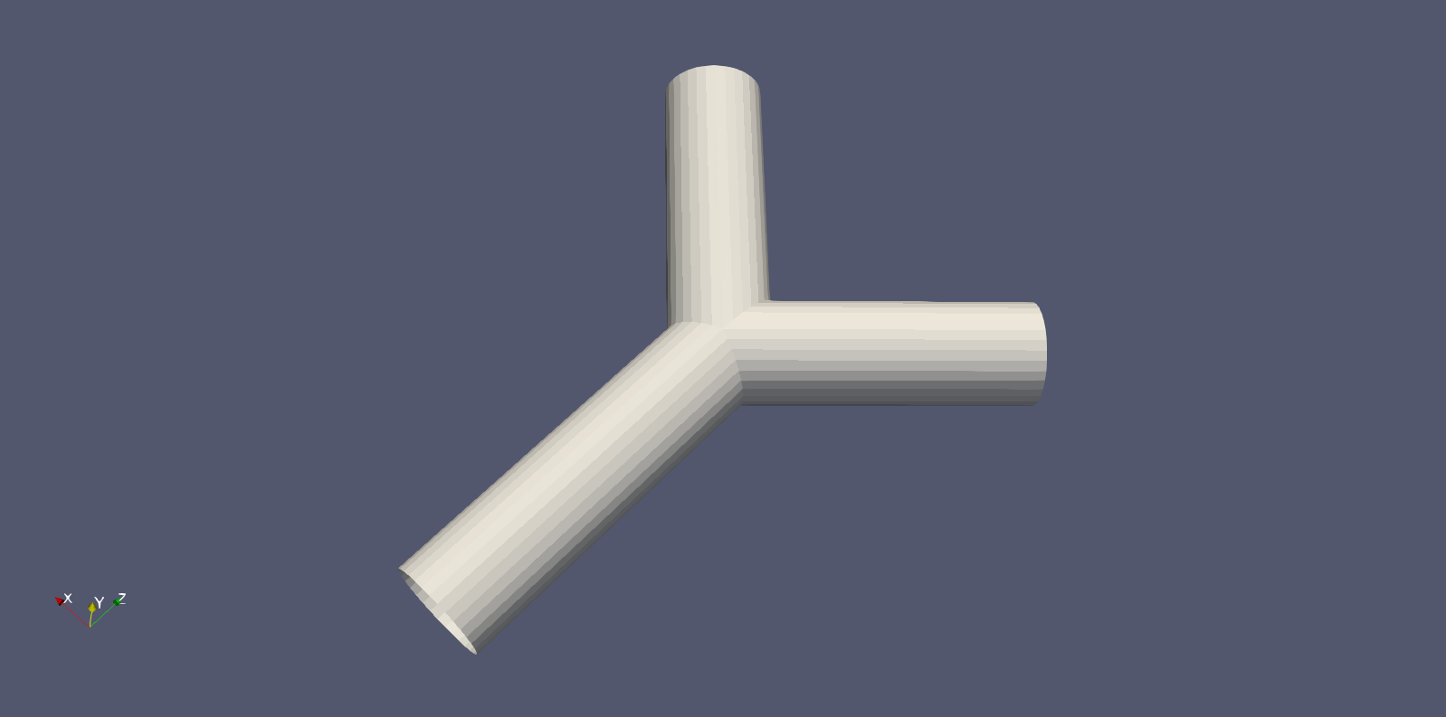
The actual geometry being run by HemeLB is specified by a geometry file, bifurcation.gmy which represents the splitting of a single cylinder into two. This can be seen as simplified representation of many vascular junctions presented throughout the network of arteries and veins.

Understanding your output files

Your job will typically generate a number of output files. Firstly, there will be job output and error files with names which have been specified in the job script. These are often denoted with the submitted job name and the job number assigned by the scheduler and are usually found in the same folder that the job script was submitted from.

In a successful job, the error file should be empty (or only contain system specific, non-critical warnings) whilst the output file will contain the screen based HemeLB output.

Secondly, HemeLB will generate its file based output in the results folder. The specific name is listed in the job script with the -o option. Here, both summary execution information and property output is contained in the folder results/Extracted. For further guide on using the hemeXtract tool please see the tutorial on the HemeLB website.

Open the file results/report.txt to view a breakdown of statistics of the HemeLB job you’ve just run.

file provides various pieces of information about the completed simulation. In particular, it includes a Problem description, Timing data and Build information.

Problem description:

Configured by file input.xml with a 2010048 site geometry.
There were 18450 blocks, each with 512 sites (fluid and solid).
Recorded 0 images.
Ran with 3 threads.
Ran for 1000 steps of an intended 1000.
With 0.000010 seconds per time step.
Sub-domains info:
rank: 0, fluid sites: 0
rank: 1, fluid sites: 1012837
rank: 2, fluid sites: 997211

The problem description section gives a number of parameters including;

• how big the geometry was (here 2010048 sites)
• how many threads (i.e. CPUs) it was run on
• the number of steps and time step size used
• how the simulation domain has been distributed between the CPUs.

Note that HemeLB is run in a master+slave configuration where one CPU is dedicated to simulation coordination and while the rest solve the problem. This is why rank 0 is assigned 0 fluid sites.

Timing data:

Timing data:
Name Local Min Mean Max
Total 172 172 172 173
Seed Decomposition 9.69e-08 9.69e-08 0.00512 0.00794
Domain Decomposition 1.71e-05 1.71e-05 0.0952 0.144
File Read 0.0301 0.0301 0.946 1.41
Re Read 0 0 0 0
Unzip 0 0 0.0931 0.141
Moves 0 0 0.0213 0.0341
Parmetis 0 0 0 0
Lattice Data initialisation 2.98 2.98 4.04 4.56
Lattice Boltzmann 0.000513 0.000513 105 158
LB calc only 0.00021 0.00021 105 158
Monitoring 0.00017 0.00017 6.5 9.83
MPI Send 0.00093 0.00093 0.00322 0.00465
MPI Wait 166 0.0747 55.5 166
Simulation total 168 168 168 168
Reading communications 0 0 0.412 0.627
Parsing 0 0 0.487 0.738
Read IO 0 0 0.00404 0.00616
Read Blocks prelim 0 0 0.00384 0.00576
Read blocks all 0 0 0.906 1.36
Move Forcing Counts 0 0 0 0
Move Forcing Data 0 0 0 0
Block Requirements 0 0 0 0
Move Counts Sending 0 0 0 0
Move Data Sending 0 0 0 0
Populating moves list for decomposition optimisation 0 0 0 0
Initial geometry reading 0 0 0 0
Colloid initialisation 0 0 0 0
Colloid position communication 0 0 0 0
Colloid velocity communication 0 0 0 0
Colloid force calculations 0 0 0 0
Colloid calculations for updating 0 0 0 0
Colloid outputting 0 0 0 0
Extraction writing 0 0 0 0

The timing section tracks how much time is spent in various process of the simulation’s initialisation and execution. Here, Local reports the time spent in the process in rank 0 and the min, mean and max columns give statistics across all CPUs used in the simulation.

Here, the Simulation total is of greatest interest as it indicates how long the simulation itself took to complete and represents total wall time less the initialisation time. This parameter is how we judge the scaling performance of the code. The other parameters are described in src/reporting/Timers.h shown below and can help to identify which section of the initialisation or computation is requiring the most time to complete:

total = 0, //!< Total time
initialDecomposition, //!< Initial seed decomposition
domainDecomposition, //!< Time spent in parmetis domain decomposition
fileRead, //!< Time spent in reading the geometry description file
reRead, //!< Time spend in re-reading the geometry after second decomposition
unzip, //!< Time spend in un-zipping
moves, //!< Time spent moving things around post-parmetis
parmetis, //!< Time spent in Parmetis
latDatInitialise, //!< Time spent initialising the lattice data
lb, //!< Time spent doing the core lattice boltzman simulation
lb_calc, //!< Time spent doing calculations in the core lattice boltzmann simulation
monitoring, //!< Time spent monitoring for stability, compressibility, etc.
mpiSend, //!< Time spent sending MPI data
mpiWait, //!< Time spent waiting for MPI
simulation, //!< Total time for running the simulation

Build information:

Build type: 
Optimisation level: -O3
Use SSE3: OFF
Built at: 
Reading group size: 2
Lattice: D3Q19
Kernel: LBGK
Wall boundary condition: BFL
Iolet boundary condition: 
Wall/iolet boundary condition: 
Communications options:
Point to point implementation: Coalesce
All to all implementation: Separated
Gathers implementation: Separated
Separated concerns: OFF

Finally, this section provides some information on the compilation options used in the executable being used for the simulation. These settings are recommended by the code developers and maintainers.

Analysing your output file

Open the file results/report.txt to view a breakdown of statistics of the HemeLB job you’ve just run.

What is your walltime, what section of the initialisation or computation is taking longest to run?

Benchmarking in HemeLB: Utilising multiple nodes

In the next section we will look at how we can use all this information to perform a scalability study, but first let us run a second benchmark, this time using more than one node

Often we need to run simulations on a larger quantity of resources than that provided by a single node. For HemeLB, this change does not require any modification to the source code to achieve. Here we can easily request more nodes for our study by changing the resources requested in the job submission scripts.

Editing the submission script

Copy the jobscript into files/2node-bif. Modify the appropriate section in your submission script so that we now utilise 2 nodes and investigate the effect of changing the requested resources in your output files.

It is important that when changing the resources requested, ensure that you also modify the execution line to use the desired resources. In SLURM, this can be automated with the $SLURM_NTASKS shortcut.

How does the walltime differ between this and the 2 and 10 core versions, what are the changes?

Scaling

Going back to our athelete example from earlier in the episode, we may have determined the conditions and done a few benchmarks on their performance over different distances, we might have learned a few things.

• how fast the athelete can run over short, medium and long distances
• the point at which the athelete can no longer perform at peak performance

In computational sense, scalability is defined as the ability to handle more work as the size of the computer application grows. This term of scalability or scaling is widely used to indicate the ability of hardware and software to deliver greater comptational power when the amount of resources is increased. When you are working on an HPC cluster, it is very important that it is scalable, i.e. that the performance doesn’t rapidly decrease the more cores/nodes that are assigned to a series of tasks.

Scalability can also be looked as in terms of parallelisation efficiency, which is the ratio between the actual speedup and the ideal speedup obtained when using a certain number of processes. The overall term of speedup in HPC can be defined with the formula Speedup = t(1)/t(N).

Here, t(1) is the computational time for running the software using one processor and t(N) is the comptational time running the software with N proceeses. An ideal situation is to have a linear speedup, equal to the number of processors (speedup = N), so every processor contributes 100% of its computational power. In most cases, as an idealised situation this is very hard to attain.

Weak scaling vs Strong scaling

Applications can be divided into either strong scaling or weak scaling applications.

For weak scaling, the problem size increases as does the number of processors. In this situation, we usually want to increase our workload without increasing our walltime, and we do that by using additional resources.

Gustafson-Barsis’ Law

Speedup should be measured by scaling the problem to the number of processes, not by fixing the problem size.

Speedup = s + p * N

where s is the proportion of the execution time spent on serial code, p is the amount of time spent on parallelised code and N is the number of processes.

For strong scaling, the number of processes is increased whilst the problem size remains the same, resulting in a reduced workload for each processor.

Amdahl’s Law

The speedup is limited by the fraction of the serial part of the software that is not amenable to parallelisation

Speedup = 1/( s + p / N )

where s is the proportion of the execution time spent on serial code, p is the amount of time spent on parallelised code and N is the number of processes.

Whether one is most concerned with strong or weak scaling can depends on the type of problem being studied and the resources available to the user. For large machines, where extra resources are relatively cheap, strong scaling ability can be more useful. This allows problems to be solved more quickly.

Determine best performance from a scalability study

Consider the following scalability plot for a random application

At what point would you consider to be peak performance in this example.

1. A: The point where performance gains are no longer linear
2. B: The apex of the curve
3. C: The maximum core count
4. None of the above

You may find that a scalability graph my vary if you ran the same code on a different machine. Why?

Solution

1. No, the performance is still increasing, at this point we are no longer achieving perfect scalability.
2. Yes, the performance peaks at this location, and one cannot get higher speed up with this set up.
3. No, peak performance has already been achieved, and increasing the core count will onlt reduce performance.
4. No, although you can run extra benchmarks to find the exact number of cores at which the inflection point truly lies, there is no real purpose for doing so.

Tying into the answer for #4, if you produce scalability studies on different machines, they will be different because of the different setup, hardware of the machine. You are never going to get two scalability studies which are identical, but they will agree to some point.

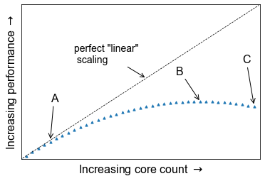
Scaling behaviour in computation is centred around the effective use of resources as you scale up the amount of computing resources you use. An example of “perfect” scaling would be that when we use twice as many CPUs, we get an answer in half the time. “Poor” scaling would be when the answer takes only 10% less time when we double the CPUs. “Bad” scaling may see a job take longer to complete when more nodes are provided. This example is one of strong scaling, where we have a fixed problem size and need to know how quickly we can solve it. The total workload doesn’t change as we increase our resources.

The behaviour of a code in this strong scaling setting is a function of both code design and hardware layout. “Good” strong scaling behaviour occurs when the time required for computing a solution outweighs the time taken for communication to occur. Less desirable scaling performance is observed when this balance tips and communication time outweighs compute time. The point at which this occurs varies between machines and again emphasise the need for benchmarking.

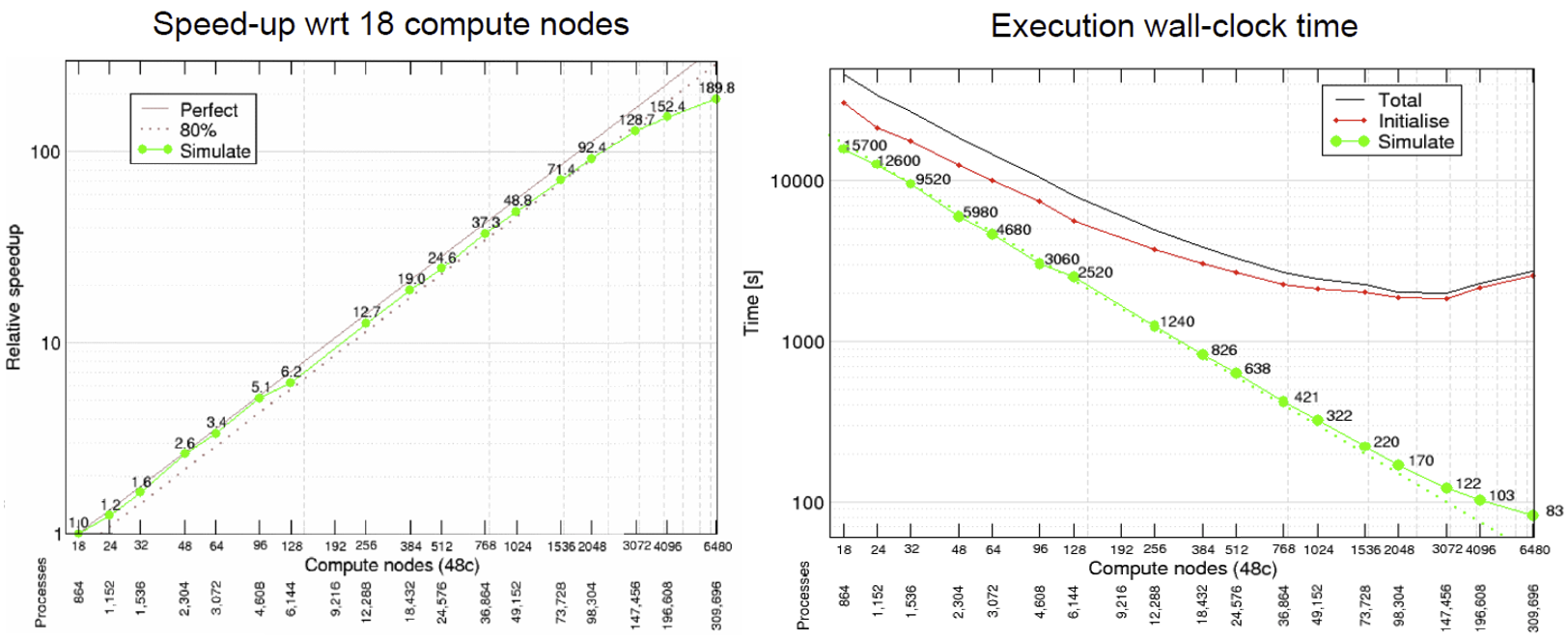
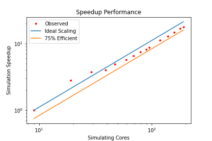
HemeLB is a code that has demonstrated very good strong scaling characteristics on several large supercomputers up to full machine scale. The plots below provide examples of such performance on the German machine SuperMUC-NG. These demonstrate how the performance varies between 864 and 309,120 CPU cores in terms of both walltime used in the simulation phase and the speed-up observed compared to the smallest number of cores used.

Plotting strong scalability

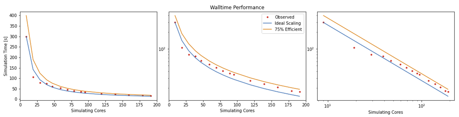
Using the original job script run HemeLB jobs at least 6 different job sizes, preferably over multiple nodes. For the size of job provided here, we suggest aiming for a maximum of around 200 cores. If your available hardware permits larger jobs, try this too up to a reasonable limit. After each job, record the Simulation Time from the Report.txt file.

Now that you have results for 2 cores, 10 cores and 2 nodes, create a scalability plot with the number of CPU cores on the X-axis and the simulation times on the Y-axis (use your favourite plotting tool, an online plotter or even pen and paper).

Are you close to “perfect” scalability?

In this exercise you have plotted performance against simulation time. However this is not the only way to assess the scalability performance of the code on your machine. Speed-up is another commonly used measure. At a given core count, the speed-up can be computed by

Speedup = SimTimeAtLeastCores/SimTimeAtCurrentCores

For a perfectly scaling code, the computational speed up will match the scale-up in cores used. This line can be used as an ‘Ideal’ measure to assess local machine performance. It can also be useful to construct a line of ‘Good’ scaling - 75% efficient for example - to further assist in performance evaluation.

Some measure of algorithmic speed can also be useful for evaluating machine performance. For lattice Boltzmann method based codes such as HemeLB, a common metric is MLUPS - Millions of Lattice site Updates Per Second, which is often expressed as a core based value and can be computed by:

MLUPS = (NumSites * NumSimulationSteps)/(1e6 * SimulationTime * Cores)

When plotted over a number of simulation size for a given machine, this metric will display a steady plateau in the regime where communication is masked by computation. When this declines, it illustrates when communication begins to take much longer to perform. The point at which this occurs will depend on the size of the geometry used and the performance characteristics of the given machine. As an illustration we have generated examples of these plots for the test bifurcation case on SuperMUC-NG. We have also illustrated the effect of different axes scaling can have on presenting scaling performance. The use of logarithmic scales can allow scaling to be easily viewed but it can also make changes in values harder to assess. Linear scales make axes easier to interpret but can also make it harder to distinguish between individual points.

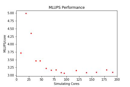
These figures also highlight two other characteristics of assessing performance. In results obtained using SuperMUC-NG, the four data points at the lowest core counts appear to have better performance than that at higher core counts. Here this is due to the the transition from one to multiple nodes on this machine and this has a consequence on communication performance. Similarly is the presence of some seemingly unusual data results. The performance of computer hardware can be occasionally variable and a single non-performant core will impact the result of the whole simulation. This emphasises the need to repeat key benchmark tests to ensure a reliable measure of performance is obtained.

Weak scaling

For weak scaling, we want usually want to increase our workload without increasing our walltime, and we do that by using additional resources. To consider this in more detail, let’s head back to our chefs again from the first episode, where we had more people to serve but the same amount of time to do it in.

We hired extra chefs who have specialisations but let us assume that they are all bound by secrecy, and are not allowed to reveal to you what their craft is, pastry, meat, fish, soup, etc. You have to find out what their specialities are, what do you do? Do a test run and assign a chef to each course. Having a worker set to each task is all well and good, but there are certain combinations which work and some which do not, you might get away with your starter chef preparing a fish course, or your lamb chef switching to cook beef and vice versa, but you wouldn’t put your pastry chef in charge of the main meat dish, you leave that to someone more qualified and better suited to the job.

Scaling in computing works in a similar way, thankfully not to that level of detail where one specific core is suited to one specific task, but finding the best combination is important and can hugely impact your code’s performance. As ever with enhancing performance, you may have the resources, but the effective use of the resources is where the challenge lies. Having each chef cooking their specialised dishes would be good weak scaling: an effective use of your additional resources. Poor weak scaling will likely result from having your pastry chef doing the main dish.

Weak scaling with HemeLB can be challenging to undertake as it is difficult to reliably guarantee an even division of work between processors for a given problem. This is due to the load partitioning algorithm used which must be able to deal with sparse and complex geometry shapes.

Key Points

• Benchmarking is a way of assessing the performance of a program or set of programs

• Strong scaling indicates how the quickly a problem of fixed size can be solved with differing number of cores on a given machine

Bottlenecks in HemeLB

Overview

Teaching: 40 min
Exercises: 45 min

Questions

• How can I identify the main bottlenecks in HemeLB?

• How do I come up with a strategy for minimising the impact of bottlenecks on my simulation?

• What is load balancing?

Objectives

• Learn how to analyse timing data in HemeLB and determine bottlenecks

• Learn how to use HemeLB compilation options to overcome bottlenecks

• Learn how to modify HemeLB file writing options to minimise I/O bottlenecks

• Learn how the choice of simulation parameters can impact the simulation time needed to reach a solution with HemeLB

How is HemeLB parallelised?

Before using accelerator packages or other optimisation strategies to speedup your runs, it is always wise to identify what are known as performance bottlenecks. The term “bottleneck” refers to specific parts of an application that are unable to keep pace with the rest of the calculation, thus slowing overall performance. Finding these can prove dfficult at times and it may turn out that only minor tweaks are needed to speed up your code significantly.

Therefore, you need to ask yourself these questions:

• Are my simulation runs slower than expected?
• What is it that is hindering us getting the expected scaling behaviour?

HemeLB distributes communicates between the multiple CPU cores taking part in a simulation through the use of MPI. One core acts as a ‘master thread’ that coordinates the simulation whilst the remaining ‘workers’ are dedicated to solving the flow through their assigned sub-domains. It is important to note that the ‘threads’ in this case are not the same as OpenMP and used as a terminology. This work pattern can generate features of a simulation that could give rise to bottlenecks in performance. Other bottlenecks may arise from one’s choice in simulation parameters whilst others may be caused by the hardware on which a job is run.

In this episode, we will discuss some bottlenecks that may be observed within the use of HemeLB.

Identify bottlenecks

Identifying (and addressing) performance bottlenecks is important as this could save you a lot of computation time and resources. The best way to do this is to start with a reasonably representative system having a modest system size and run for a few hundred/thousand timesteps, small enough so that it doesn’t run for too long, but large enough and representative enough that you can project a full workflow.

Benchmark plots - particularly for speed-up and MLUPS/core - can help identify when a potential bottleneck becomes a problem for efficient simulation. If an apparent bottleneck is particularly significant, timing data from a job can also be useful in identifying where the source of it may be. HemeLB has a reporting mechanism that we introduced in the previous episode that provides such information. This file gets written to results/report.txt. This file provides a wealth of information about the simulation you have conducted, including the size of simulation conducted and the time spent in various sections of the simulation.

We will discuss three common bottlenecks that may be encountered with HemeLB:

• Load balance
• Writing data
• Choice of parameters

In some circumstances, the options available to overcome the bottleneck may be limited. But they will provide insight into why the code is performing as observed, and can also help to ensure that accurate results are obtained.

Load balancing

One important issue with MPI-based parallelization is that it can under-perform for systems with inhomogeneous distribution of work between cores. It is pretty common that the evolution of simulated systems over time begin to reflect such a case. This results in load imbalance. While some of the processors are assigned with a finite number of lattice sites to deal with for such systems, a few processors could have far fewer sites to update. The progression of the simulation is held up by the core with the most work to do and this results in an overall loss in parallel efficiency if a large imbalance is present. This situation is more likely to expose itself as you scale up to a large large number of processors for a fixed number of sites to study.

Quantifying load imbalance

A store has 4 people working in it and each has been tasked with loading a number of boxes. Assume that each person fills a box every minute.

Person	James	Holly	Sarah	Mark	Total number of boxes
Number of boxes	6	1	3	2	12

1. How long would it take to finish packing the boxes?
2. If the work is evenly distributed among the 4 people how long would it take to fill up the boxes?

Solution

1. It would take 6 minutes as James has the most number of boxes to fill. This means that Holly will have been watching for 5 minutes, Sarah for 3 and Mark for 2.
2. If the work was distributed evenly, (# boxes/# people), then it would take 3 minutes to complete. Load balancing works in such a way that if a core is underutilised, it takes some work away from other ones to complete the task more quickly. This is particularly useful in chemistry/biological systems where a large area is left with little to do.

In the HemeLB results file, the number of sites assigned to each core is reported near the top of the file and can be used to check for signs of significant imbalance between cores. For example we plot below how HemeLB has distributed the workload of the bifurcation geometry on 48 and 192 cores. Note in both cases that rank 0 has no sites assigned to it. As the speed of a simulation is governed by the core with the most work to do, we do not want to see a rank that has significantly more sites than the others. Cores with significantly less workload should not hold up a simulation’s progression but will be waiting for other cores to complete and thus wasting its computational performance potential. The success of a distribution will depend on the number of cores requested and the complexity of the domain.

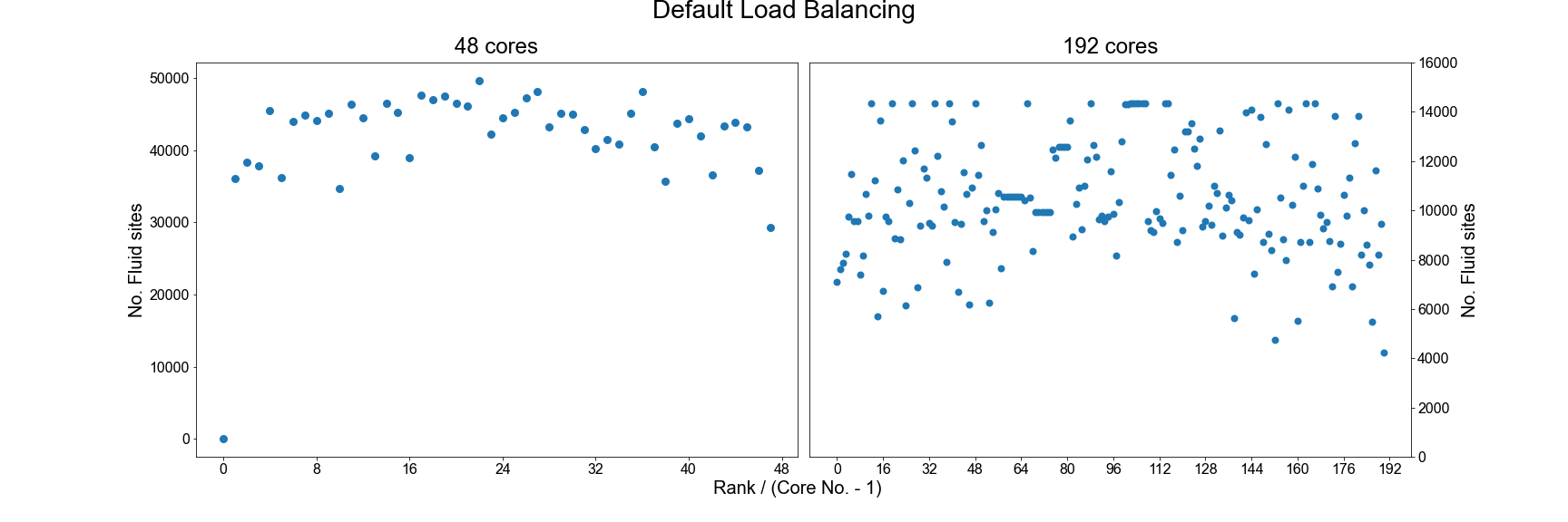
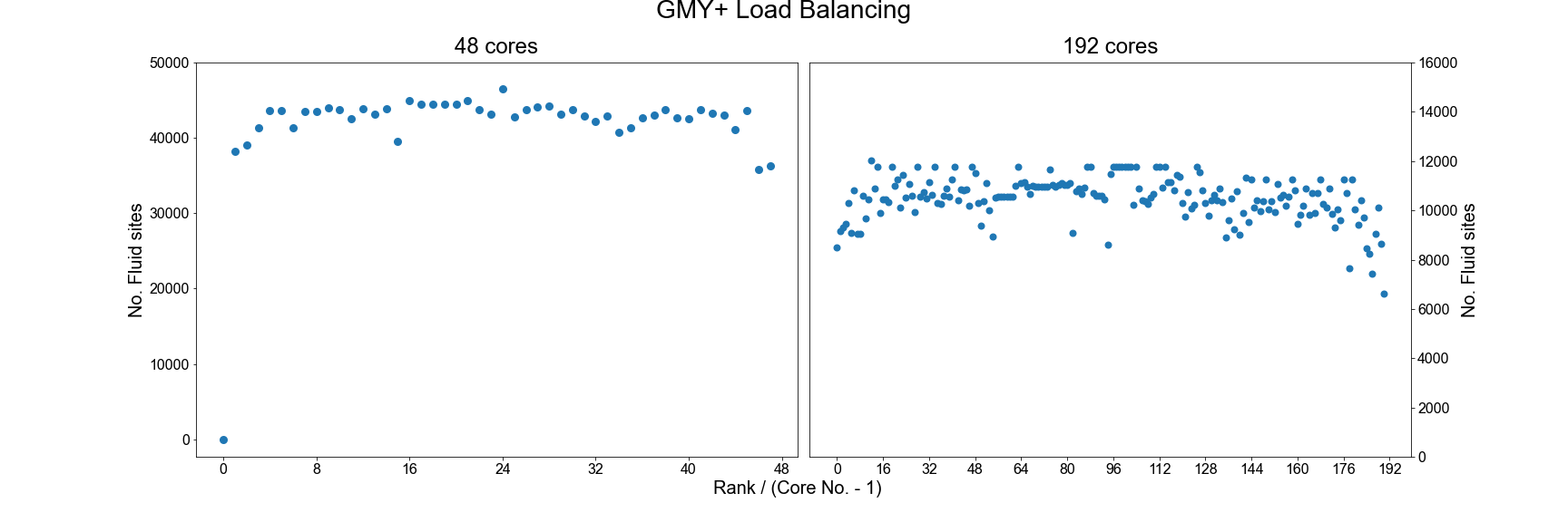
In general, the default load distribution algorithm in HemeLB has demonstrated good performance except in extreme circumstances. This default algorithm however does assume that each node type: Bulk fluid, Inlet, Outlet, Wall; all require the same amount of computational work to conduct and this can generate imbalance, particularly when there are a large number of non-bulk sites present in a geometry. HemeLB has a tool available to help correct this imbalance by assigning weights to the different site types in order to generate a more even distribution, this converts the geometry data format from *.gmy to *.gmy+.

Compiling and using gmy2gmy+

Download the code for the gmy2gmy+ converter from files/gmy2gmy+ along with its corresponding Makefile and compile it on your machine. This script is run with the following instruction (where DOMAIN is your test domain name, eg. bifurcation.gmy):

./gmy2gmy+ DOMAIN.gmy DOMAIN.gmy+ 1 2 4 4 4 4 

This assigns a simple weighting factor of 1 to fluid nodes, 2 to wall nodes and 4 to variants of in/outlets (in order: Inlet, Outlet, Inlet+Wall, Outlet+Wall).

Recompile HemeLB so that it knows to read gmy+ files. To keep your old executable, rename the build folder to build_DEFAULT, so you can have a buildGMYPLUS directory for two executables. Edit the build script in buildGMYPLUSto change the flag from OFF to;

-DHEMELB_USE_GMYPLUS=ON

Use the tool to convert bifurcation.gmy into the new gmy+ format.

An example of the improved load balance using the gmy+ format are shown below:

Testing the performance of gmy+

Repeat the benchmarking tests conducted in the previous episode using the gmy+ format. Rename the results folder previously created to a folder name of your choice to keep your old results. You will also need to edit the input.xml file accordingly) and compare your results. Also examine how load distribution has changed as a result in the report.txt file.

Try different choices of the weights to see how this impacts your results.

Using the ParMETIS library

Another option for improving the load balance of HemeLB is to make use of the ParMETIS library that was built as a dependency in the initial compilation of the code. To do this you will need to recompile the source code with the following option enabled: -DHEMELB_USE_PARMETIS=ON. This tool takes the load decomposition generated by the default HemeLB algorithm and then seeks to generate an improved decomposition.

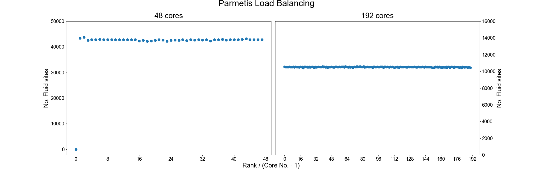
As can be seen, using ParMETIS can generate a near perfect load distribution. Whilst this may seem like an ideal solution it does come with potential drawbacks.

1. Memory Usage: Some researchers have noted that ParMETIS can demand a large amount of memory during its operation and this can become a limiting factor on its use as domains become larger.
2. Performance Improvement: With any of the suggested options for improving load balance, it is important to assess how much performance gain has been achieved through this change. This should be assessed in two metrics: 1) Simulation Time: This looks at the time taken for the requested iterations to complete and is the value used for assessing scaling previously. 2) Total Walltime: Includes both the Simulation Time and the time needed to initialise the simulation. The use of extra load balancing tools requires the extra initialisation time and it needs to be judged whether this extra cost is merited in terms of the achieved improvement in Simulation Time.

As many HPC systems charge for the Total Walltime of a job, it is inefficient to use a tool that causes this measure to increase. For small geometries, the initialisation time of HemeLB can be very quick (a few seconds) but for larger domains with multiple boundaries, this can extend to tens of minutes.

Testing the performance of gmy+ and ParMETIS

Repeat the benchmarking tests conducted in the previous episode using the gmy+ and ParMETIS. Once again, rename the results folder so you can keep the original and gmy+ simualtion results. Similarly, edit the input.xml file so that it is looking for the gmy+ file when testing this, save as a separate file; when testing ParMETIS the original input.xml file can be used and compare your results.

You should also spend some time examining how load distribution has changed as a result in the report.txt file.

Try different choices of the gmy+ weights to see how this impacts your results. See how your results vary when a larger geometry is used (see files/biggerBif for gmy and input files).

Example Results

Note that exact timings can vary between jobs, even on the same machine - you may see different performances. The relative benefit of using load balancing schemes will vary depending on the size and complexity of the domain, the length of your simulation and the available hardware.

Scheme	Cores	Initialisation Time (s)	Simulation Time (s)	Total Time (s)
Default	48	0.7	56.0	56.7
Default	192	1.0	15.3	16.3
GMY+	48	0.7	56.1	56.8
GMY+	192	1.0	13.2	14.2
ParMETIS	48	2.6	56.7	59.3
ParMETIS	192	2.4	12.5	14.9

Data writing

With all simulations, it is important to get output data to assess how the simulation has performed and to investigate your problem of interest. Unfortunately, writing data to disk is a cost that can negatively impact on simulation performance. In HemeLB, output is governed by the ‘properties’ section of the input file.

 <properties>
    <propertyoutput file="whole.dat" period="1000">
      <geometry type="whole" />
      <field type="velocity" />
      <field type="pressure" />
    </propertyoutput>
    <propertyoutput file="inlet.dat" period="100">
      <geometry type="inlet" />
      <field type="velocity" />
      <field type="pressure" />
    </propertyoutput>
    <propertyoutput file="outlet.dat" period="100">
      <geometry type="inlet" />
      <field type="velocity" />
      <field type="pressure" />
    </propertyoutput>
  </properties>
</hemelbsettings>

In this example, we output pressure and velocity information at the inlet and outlet surfaces of our domain every 100 steps and for the whole simulation domain every 1000 steps. This data is written to compressed *.dat files in results/Extracted. It is recommended that the whole option is used with caution as it can generate VERY large *.dat files. The larger your simulation domain, the greater the effect of data writing will be.

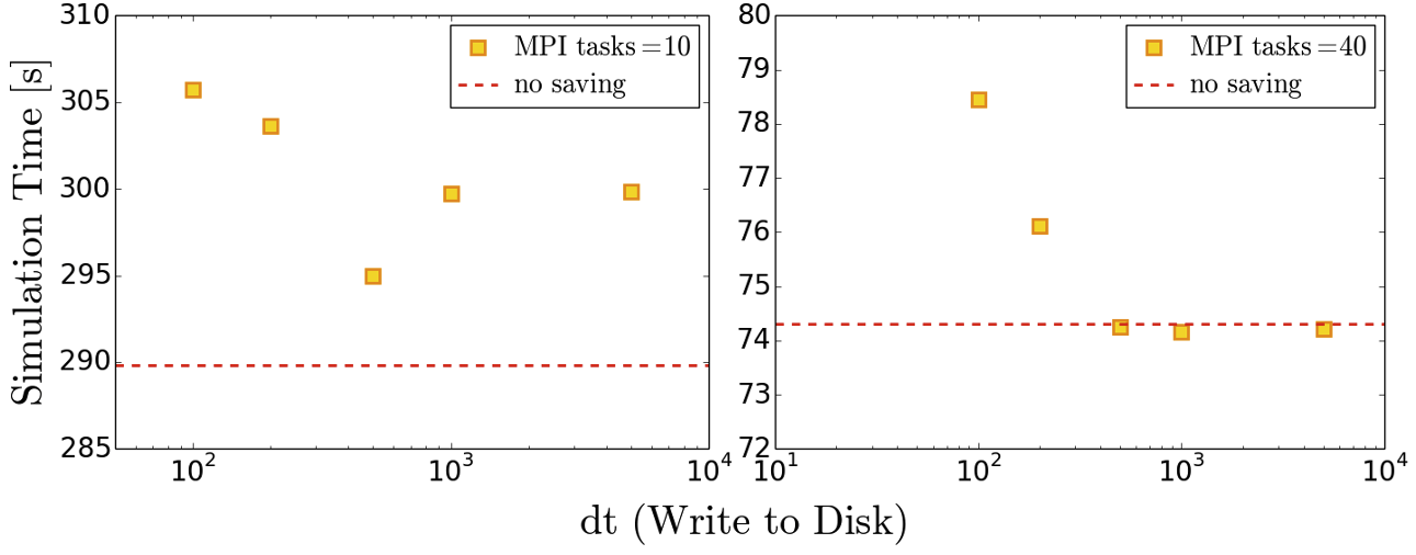
Testing the effect of data writing

Repeat the benchmarking tests conducted in the previous episode now outputting inlet/outlet and whole data at a number of different time intervals. Compare your results to those you have previously obtained. Given output is critical to the simulation process what would be a suitable strategy for writing output data?

Below we provide some example results obtained on SuperMUC-NG by writing the whole data set at different time intervals. The impact on performance is clear to observe.

Effect of model size

In files/biggerBif you can find a higher resolution model ( ≈ 4 times larger) of the bifurcation model we have been studying. Repeat some of the exercises on load balancing and data writing to see how a larger model impacts the performance of your system.

Choice of simulation parameters

With most simulation methods, results that accurately represent the physical system being studied can only be achieved if suitable parameters are provided. When this is not the case, the simulation may be unstable, it may not represent reality or both. Whilst the choice of simulation parameters may not change the algorithmic speed of your code, they can impact how long a simulation needs to run to represent a given amount of physical time. The lattice Boltzmann method, on which HemeLB is based, has specific restrictions that link the discretization parameters, physical variables and simulation accuracy and stability.

In these studies, HemeLB is using a single relaxation time (or BGK) collision kernel to solve the fluid flow. HemeLB (and the lattice Boltzmann method more widely) also has other collision kernels that can permit simulation of more sophisticated flow scenarios such as non-Newtonian fluid rheology or possess improved stability or accuracy characteristics. The BGK kernel is typically the first choice for the collision model to used and is also simplest (and generally fastest) to implement and perform computationally. In this model viscosity, lattice spacing, and simulation timestep are related to the relaxation parameter τ by,

ν = ¹/₃(τ - ½) ^Δx2/_Δt

Here:

• ν - Fluid viscosity [m²/s] - in HemeLB this is set to 4x10^-6 m²/s the value for human blood
• Δx - Lattice spacing [m]
• Δt - Time step [s]

This relationship puts physical and practical limits on the values that can be selected for these parameters. In particular, τ > ½ must be imposed for a physical viscosity to exist, values of τ very close to ½ can be unstable. Generally, a value of τ ≈ 1 gives the most accurate results.

The lattice Boltzmann method can only replicate the Navier-Stokes equations for fluid flow in a low Mach number regime. In practice, this means that the maximum velocity of the simulation must be significantly less than the speed of sound of the simulation. As a rough rule of thumb, the following is often acceptable in simulations (though if smaller Ma can be achieved, this is better):

Ma = ^(3u_max*Δt)⁄_Δx

Often the competing restrictions placed on a simulation by these two expressions can demand a small time step to be used.

Determining your physical parameters

Suppose you wish to simulate blood flow through a section of the aorta with a maximum velocity of 1 m/s for a period of two heartbeats (2 seconds). Using the expressions above, determine suitable choices for the time step if your geometry has a grid resolution of Δx = 100 μm.

How many iterations do you need to run for this choice? How do your answers change if you have higher resolutions models with (i) Δx = 50 μm and (ii) Δx = 20 μm? What would be the pros and cons of using these higher resolution models?

Solution

Starting points would be the following, these would likely need further adjustment in reality:

• For Δx = 100 μs, Δt = 5 μs gives Ma ≈ 0.087 and τ = 0.506; 400,000 simulation steps required
• For Δx = 50 μs, Δt = 2.5 μs gives Ma ≈ 0.087 and τ = 0.512; 800,000 simulation steps required
• For Δx = 20 μs, Δt = 1 μs gives Ma ≈ 0.087 and τ = 0.530; 2,000,000 simulation steps required

Higher resolution geometries have many more data points stored within them - halving the grid resolution requires approximately 8x more points and will take roughly 16x longer to simulate for the same Ma and physical simulation time. Higher resolution domains also generate larger data output, which can be more challenging to analyse. The output generated should also be a more accurate representation of the reality being simulated and can achieve more stable simulation parameters.

Key Points

• The best way to identify bottlenecks is to run different benchmarks on a smaller system and compare it to a representative system

• Effective load balancing is being able to distribute an equal amount of work across processes.

• Evaluate both simulation time and overall wall time to determine if improved load balance leads to more efficient performance.

• The choice of simulation parameters impacts both the accuracy and stability of a simulation as well as the time needed to complete a simulation. This is especially true for solvers using explicit techniques such as HemeLB.

• For all applications, writing data to file can be a time consuming activity. Carefully consider what data you need for post-processing to minimise the time spent in this regime.

Accelerating HemeLB

Overview

Teaching: 30 min
Exercises: 90 min

Questions

• What are the various options to accelerate HemeLB?

• What accelerator tools are compatible with which hardware?

Objectives

• Understand the different methods of accelerating a HemeLB simulation

• Learn how to invoke the different accelerator packages across different hardwares

• Understand the risks of trying to naively use HemeLB acceleration methods on a new domain or machine

How can I accelerate HemeLB performance?

There are two basic approaches to accelerate HemeLB simulations that we will discuss in this episode. How successful these will be will depend on the hardware that you have available and how well you know the characteristics of the simulation problem under investigation.

Versions of HemeLB that are accelerated by GPUs are also available and these can yield significant speed-up compared to the CPU code. We will discuss the use of these further in the next episode.

The two options we will discuss in this episode are:

• 1) Vectorisation
• 2) Monitoring

Vectorisation overview

At the heart of many simulation codes will be a relatively small number of kernels that are responsible for the key problem solving steps. In the lattice Boltzmann method of HemeLB it is the update of the fundamental population distributions and the conversion of these to macroscopic properties of interest. When these kernels are written in code, they are often written in variables of the type ‘double’ that may be naively acted on in a sequential manner. However modern processors can operate on multiple ‘double’ sized units of memory at the same time - the latest Intel cores can operate on eight at once. Therefore significant speed-ups can be obtained by invoking parallelism at this fundamental level by adjusting the instructions of this fundamental kernel to allow vector operations. Modern compilers can often do a lot of this without having to write specific code to act in this fashion. However, sometimes code complexity can mean that this is not fully achieved by the compiler and vectorised code needs to be written. This is done through the use of intrinsic instructions that explicitly tell the compiler how a certain portion of code should be compiled.

In HemeLB, the key computational kernels have been encoded with SSE3 intrinsics that allows two ‘double’ units to be operated on simultaneously. This level of optimisation should be compatible with most modern CPUs, even those available on desktops and laptops. To enact this in HemeLB set the -DHEMELB_USE_SSE3 flag in the compilation script to ON and recompile. HemeLB can also use AVX2 intrinsics where the instructions can operate on four ‘double’ units to be acted on with a single instruction. This can be enabled by setting -DHEMELB_USE_AVX2 to ON and the SSE3 flag to OFF. Before trying this, be certain that your CPU is able to use AVX2 intrinsics. The encoding of the key kernels using the intrinsics can be seen in the file src/lb/lattices/Lattice.h. In src/CMakeLists.txt you can identify the compiler flags that are imposed when SSE3 or AVX2 instrinsics are implemented. These options can also allow the compiler to implicitly vectorise some other sections of the code, however the performance of this alone has not been seen to match that obtained when the explicit intrinsics are used for the key computational kernels.

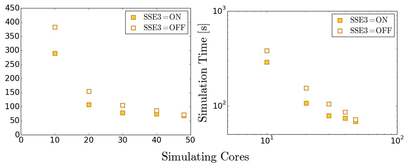
Case Study: Simulation acceleration with intrinsics

Repeat your scaling benchmark tests with SSE3 intrinsics active and compare performance against that achieved with the ‘naive’ code implementation and default compiler options. In particular, note how walltime and parallel efficiency (speed_up_compared_to_smallest/core_scale_up) changes with their use.

Example Results

Note that exact timings can vary between jobs, even on the same machine - you may see different performance. The benefit of using intrinsics can become more apparent at higher core counts, longer runtimes and larger domains.

Scheme	Cores	Initialisation Time (s)	Simulation Time (s)	Total Time (s)
Basic	48	0.7	67.5	68.2
Basic	192	1.0	19.6	20.6
SSE3	48	0.7	56.1	56.8
SSE3	192	1.0	15.2	16.2
AVX2	48	0.7	55.9	56.6
AVX2	192	1.1	14.9	16.0

Monitoring in HemeLB

In the input file provided for the benchmarking case, you will notice the following section:

<monitoring>
<incompressibility/>
</monitoring>

This makes the HemeLB simulation monitor for numerical characteristics that will cause the simulation to become irretrievably unstable and aborts the simulation at this point. This process checks the data at every site in the domain at every time step. As simulation domains grow, this can become a significant portion of the computational time. If you are studying a simulation domain with boundary that are known two generate stable and sensible results, deactivating this feature can reduce the time needed for a simulation to complete. It is STRONGLY recommended to keep this feature active for new domains and boundary conditions to be aware of when simulations are unstable or are possibly on the verge of becoming so. Stability monitoring can be removed by deleting this section or commenting it out via:

<!-- <monitoring>
<incompressibility/>
</monitoring> -->

Case Study: Reduced runtimes without stability monitoring

Repeat the benchmarking tests case for both geometry sizes the with the stability monitoring deactivated. Compare how significant the effect of stability monitoring is for the larger domain.

Another monitoring option that can be introduced to your simulation is a check to observe when steady-state is reached. HemeLB is a explicit solver meaning that it is not ideally suited to steady-state simulations as implicit methods can be. Once a suitable timestep is determined the simulation will continuously step through time until the desired number of iterations is completed. Unfortunately, it is not always possible to know in advance how many iterations are required for steady-state to be reached. This monitoring check will automatically terminate a simulation once a stipulated tolerance value on velocity is reached. This is invoked in the input file by:

<monitoring>
<incompressibility/>
    <steady_flow_convergence tolerance="1e-3" terminate="true" criterion="velocity">
          <criterion type="velocity" units="m/s" value="1e-5"/>
  </steady_flow_convergence> 
</monitoring>

The value for the velocity stated here is the reference value against which the local error is compared.

Case Study: Reduced runtimes for convergence

Repeat the benchmarking test case with the convergence monitoring in place. By how much is the simulation truncated? Try different values for tolerance and input boundary conditions. NB: Steady-state convergence will not work accurately or reliably for intentionally transient flow conditions.

Tuning MPI Communications

Depending on your systems, another option that may yield performance gains is in the modification of how the underlying MPI communications are managed. For general operation however, the default settings provided in the compilation options for HemeLB have been found to work very well in most applications. For the curious reader, the available compilation options are:

Case Study: Demonstration of MPI Setting Choices

To demonstrate the impact of changing MPI options, each were individually examined in turn with all other flags remaining in their default setting. Further discussion on MPI implementation techniques can be found on resources such as https://mpitutorial.com/tutorials/ among many others.

Example Results

Note that exact timings can vary between jobs, even on the same machine - you may see different performance. Here it can be seen that the use of some options in isolation can prevent HemeLB from successfully operating, whilst those with successfult execution only saw variation of performance within the expected variability of machine operation. As an exercise see whether such behaviour is repeated, and occurs consistently, on your local machine.

Scheme	Option	Initialisation Time (s)	Simulation Time (s)	Total Time (s)
All default options	Defaults	0.7	67.0	67.7
-DHEMELB_POINTPOINT_IMPLEMENTATION	'Separated'	0.7	67.3	68.0
-DHEMELB_POINTPOINT_IMPLEMENTATION	'Immediate'	Job Failed	-	-
-DHEMELB_GATHERS_IMPLEMENTATION	'ViaPointPoint'	Job Failed	-	-
-DHEMELB_ALLTOALL_IMPLEMENTATION	'ViaPointPoint'	Job Failed	-	-
-DHEMELB_SEPARATE_CONCERNS	ON	0.7	66.2	66.9

Key Points

• The use of efficiently vectorised instructions can effectively speed-up simulations compared to default options, however they may not be available on all CPUs

• Simulation monitoring in HemeLB can require a significant amount of time to complete. If a set of simulation parameters is known to be stable and acceptably accurate, removal of this feature will accelerate simulation time. It is recommended to be kept in place to catch unstable simulations when new geometries or simulation parameters are being investigated.

GPUs with HemeLB

Overview

Teaching: 15 min
Exercises: 15 min

Questions

• Why do we need GPUs?

• What is CUDA programming?

• How is GPU code profiled?

• How do I use the HemeLB library on a GPU?

• What is the performance like?

• What is a 1-to-1, 2-to-1 relationship in GPU programming

Objectives

• Understand and implement basic concepts of GPUs and CUDA

• Implement HemeLB using a GPU

Why do we need GPUs?

A Graphics Processing Unit (GPU) is a type of specialised processor originally designed to accelerate graphics rendering, this includes video games. GPUs can have thousands of cores, which can perform tasks simultaneously, which at the time was very helpful for creating pixels on a screen for gaming purposes.

Imagine you were playing a game using a CPU, which only has a handful of cores, compared to a GPU, which has thousands, you can get an idea why a GPU is more fit for purpose in that way. However, it was gradually realised that a GPU can also be used to accelerate other types of calculations as well, involving massive amounts of data, due to the way that it is designed to operate.

Top level GPUs nowadays, such as the NVIDIA A100 GPU has 6912 CUDA cores and 432 Tensor cores. A CUDA core is the NVIDIA version of a CPU core, and which can run CUDA code. A Tensor core is a more advanced core which is fundamental to AI and deep learning workflows, using such libraries as (TensorFlow)[https://www.tensorflow.org/]. We will not discuss any further differences between these two now, but what you need to remember and understand is that a GPU has much more processing power than a CPU to complete a given task.

If you need to perform a task on massive amounts of data, then the same analysis (calculations - set of code) will be executed on/for each one of the elements/data that we have. A CPU would have to go through each one of the elements in a serial manner, i.e. perform the analysis on the first element, once finished move to the next one and so on and so forth, until it manages to process everything. A GPU on the other hand, will do this in parallel (large scale parallelism), depending on how may cores it has. The same mathematical function will run over and over again but at a large scale, offering significant speed-up to the calculations.

A nice demonstration of the above was given by the MythBusters at an NVIDIA conference in 2008. Although it is a big oversimplication of the internal processes and communications between a CPU and a GPU, it gives an ideal as to why GPUs are regarded so highly.

Hence, in scientific computing, with GPUs we can achieve massive acceleration of our calculations. That is why GPUs are becoming commonplace on high-end HPC machines, with a number of GPUs installed on each node.

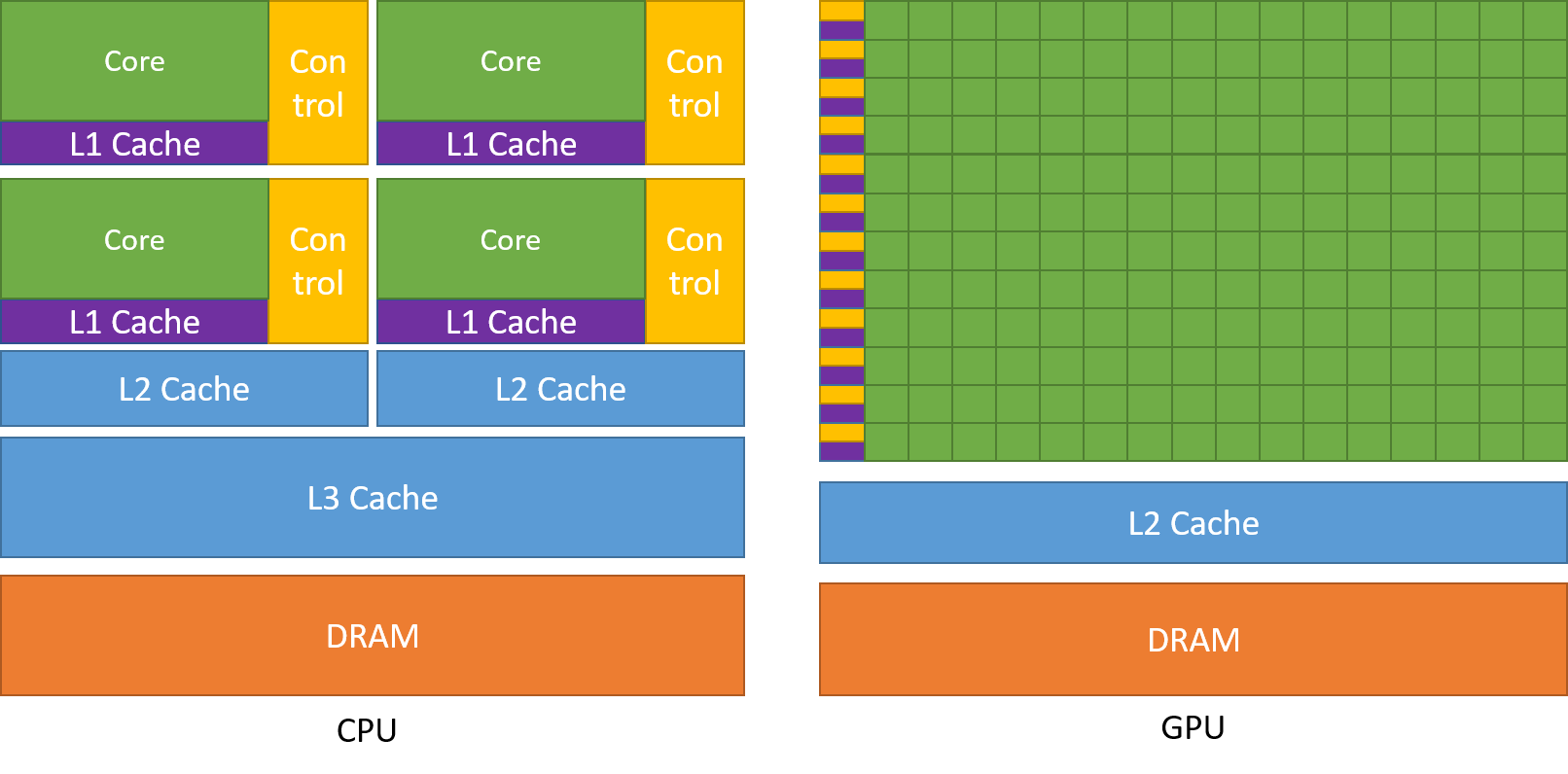
The schematic Figure from NVIDIA documentation shows an example distribution of chip resources for a CPU versus a GPU.

It is worth noting however that even though GPUs have more cores than a CPU, and can technically do things much quicker, their main disadvantage is their low memory, and this limits them to doing small, albeit vast amounts of smaller calculations at once. So you would not want to have a GPU running a long and complex calculation on a single core, as it will likely run out of memory and waste using a GPU in the first place, therefore a CPU is more practical.

CPUs vs GPUs

Look at the table below on the main differences between CPUs and GPUs. Some of these values are true and some are false. Spend a few minutes sorting through them to match the answer to the correct column.

CPU	GPU
Central Processing Unit	Graphics Processing Unit
Many cores	Several cores
Low latency	High throughput
Good for parallel processing	Good for serial processing
Handful of operations at once	Thousands of operations at once
Consumes/needs more memory	Requires less memory
Lower speed	Higher speed
Weak cores	Powerful cores
Complements main brain to perform calculations	Considered as main ‘brain’ of computer
Explicit management of threads	Threads managed by hardware
Data Parallelism	Task Parallelism
Few highly optimised instructions	Diverse instruction sets

Solution

CPU	GPU
Central Processing Unit	Graphics Processing Unit
Several cores	Many cores
Low latency	High throughput
Good for serial processing	Good for parallel processing
Handful of operations at once	Thousands of operations at once
Consumes/needs more memory	Requires less memory
Lower speed	Higher speed
Powerful cores	Weak cores
Considered as main ‘brain’ of computer	Complements main brain to perform calculations
Explicit management of threads	Threads managed by hardware
Task Parallelism	Data Parallelism
Diverse instruction sets	Few highly optimised instructions

CUDA Programming Basics

The most important concept to have in mind when it comes to CUDA and GPU programming, is that the compute intensive parts of a code can be ported onto the GPU (device) for the calculations to take place for a fraction of the time it would take to complete on a CPU. Following that, the results are then returned back to the CPU (host). Hence, the developer needs to implement what are known as GPU CUDA kernels, which are the functions for doing the calculations on the GPU, but also arrange:

• the data transfers to and from the GPU, as well as
• the synchronisation points, i.e. when to stop the code moving past a given point until a certain task on the GPU has been completed.

With the above in mind, a typical workflow for a CUDA C++ program is:

1. Declare and allocate host (CPU) and device (GPU) memory.
2. Initialize host (CPU) data.
3. Transfer data from the host (CPU) to the device (GPU).
4. Execute one or more CUDA kernels (the computations to be performed on the GPU).
5. Transfer results from the device (GPU) back to the host (CPU).

GPU CUDA kernel - CUDA function

CUDA programming can take a bit to get used to and as yet there are no Carpentries style resources for CUDA programming available, however here we will provide a brief lookover at the main functionalities and differences.

The specifier __global__ is added in front of the function, which tells the CUDA C++ compiler that this is a function that runs on the GPU and can be called from CPU code. The remainder of the code will be relatively similar, however when you are defining your function, the keyword will be required to run the function on a GPU. A full example of defining a GPU CUDA kernel would be as follows;

__global__ void GPU_Cuda_Kernel_Name(kernel's_arguments)

GPU Memory Hierarchy - Memory Allocation in CUDA

Before we carry onto how to launch a kernel, we need to discuss the memory hierarchy of a GPU, as an understanding of it is crucial to getting a CUDA code to actually run and work. In CUDA, the kernel is executed with the aid of CUDA threads, arranged in groups (blocks). Each thread is given a unique thread ID, which is accessible within the GPU kernel through built-in variables. CUDA defines the following built-in variables: blockDim, blockIdx, and threadIdx, which are predefined variables of type dim3. blockDim contains the dimensions of each thread block, while threadIdx and blockIdx contain the index of the thread within its thread block and the thread block within the grid of blocks, respectively.

Using the thread’s index we can access different GPU memory locations, either for loading or writing data.
Each thread has also a private local memory. NVIDIA’s documentation page gives a good overview.

One thread is never enough though when dealing with GPUs, as threads come in thread blocks, which can be executed in serial or parallel. Depending on the GPU you are utilising, a thread block can contain a maximum of either 512 or 1024 of these threads.

Each thread block has shared memory visible to all threads of the block and with the same lifetime as the block. All threads have access to the same global memory. An overview of the memory Hierarchy is outlined below.

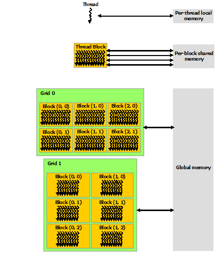
Launching the GPU kernel

The GPU CUDA kernel is launched by using a specific syntax, the triple angle bracket <<< >>>. This will inform the compiler that the kernel that follows is a GPU kernel and will therefore be executed on the GPU. The information between the triple angle brackets is the execution configuration, which determines how many threads on the device (GPU) will execute the kernel in parallel. These threads are arranged in what are thread blocks, hence the developer should specify how many threads there are per block. The number of threads per block should be a round multiple of 32 (the warp size).

An example of a launching a GPU CUDA kernel (GPU_Cuda_Kernel_Name) is as follows:

// Cuda kernel set-up
int nThreadsPerBlock = 128; //Number of threads per block
dim3 nThreads(nThreadsPerBlock);
 
// Number of BLOCKS needed 
int nBlocks = (number_of_Elements)/nThreadsPerBlock	+ ((number_of_Elements % nThreadsPerBlock > 0) ? 1 : 0);

// Launch the GPU CUDA kernel
GPU_Cuda_Kernel_Name <<< nBlocks, nThreads >>> (Provide_Arguments_here); 

The first argument in the execution configuration; GPU_Cuda_Kernel_Name <<< nBlocks, nThreads>>> specifies the number of thread blocks (nBlocks), while (nThreads) specifies the number of threads in a thread block.

Remember that CUDA kernel launches don’t block the calling CPU thread. This means that once the kernel is launched, the control is returned to the CPU thread and the code will resume. In order to ensure that the GPU kernel has completed its task, a synchronsation barrier might be needed using cudaDeviceSynchronize().

NVIDIA’s website provides plentiful discussions and simple examples and guides on the NVIDIA CUDA Toolkit. We will not go into durther details, however please feel free to check these out in your own time

CUDA Streams and Concurrency

A CUDA kernel when launched is placed in the default CUDA stream. A CUDA stream is like an execution path. All operations in the same stream need to be completed and executed in order, before moving forward.

It is also possible, however, to launch kernels in different CUDA streams and by doing so these kernels may execute out of order with respect to one another or concurrently. An example of a launching a GPU CUDA kernel (GPU_Cuda_Kernel_Name) in a specified CUDA stream (name of stream CUDA_stream_ID) is provided here:

// Launch the GPU CUDA kernel in stream CUDA_stream_ID
GPU_Cuda_Kernel_Name <<< nBlocks, nThreads, 0, CUDA_stream_ID >>> (Provide_Arguments_here); 

Data Transfers in CUDA C/C++

As mentioned above, when performing calculations on the GPU, memory needs to be allocated onto the GPU (cudaMalloc()); then data that will be processed needs to be copied from the host to the device (cudaMemcpyHostToDevice), perform the calculations (execute the CUDA kernels on the device/GPU) and finally copy the results from the device to the host (cudaMemcpyDeviceToHost). Data transfers are performed using cudaMemcpy function. The syntaxt of cudaMemcpy is as follows:

cudaMemcpy(void *dst, void *src, size_t count, cudaMemcpyKind kind)

cudaMemcpyKind is either cudaMemcpyHostToDevice or cudaMemcpyDeviceToHost. The 2 possible kinds of CUDA memory copies are:

a. H2D: from the Host (CPU) to the Device (GPU)

cudaMemcpy(d_A, h_A, size_of_h_A_in_Bytes, cudaMemcpyHostToDevice)

b. D2H: from the Device (GPU) to the Host (CPU)

cudaMemcpy(h_A, d_A, size_of_d_A_in_Bytes, cudaMemcpyDeviceToHost)

These memory copies can be Synchronous (as above) or Asynchronous (cudaMemcpyAsync). In the case of asynchronous memory copy, the developer should provide the CUDA stream as a last argument to the cudaMemcpyAsync function call. This allows overlapping the memory copies with other operations (kernels or mem.copies) on the GPU running on different CUDA streams.

Simple CUDA code example

Here, we provide a simple example of a CUDA code. It contains the main features discussed above: allocate input vectors in host memory and initialise them, allocate memory on the GPU, memory copies (H2D and D2H), defining and launching a GPU CUDA kernel.

• D2H: from the Device (GPU) to the Host (CPU)
• H2D: from the Host (CPU) to the Device (GPU)

// Device code
__global__ void VecAdd(float* A, float* B, float* C, int N)
{
    int i = blockDim.x * blockIdx.x + threadIdx.x;
    if (i < N)
        C[i] = A[i] + B[i];
}
            
// Host code
int main()
{
    int N = ...;
    size_t size = N * sizeof(float);

    // Allocate input vectors h_A and h_B in host memory
    float* h_A = (float*)malloc(size);
    float* h_B = (float*)malloc(size);

    // Initialize input vectors
    ...

    // Allocate vectors in device memory
    float* d_A;
    cudaMalloc(&d_A, size);
    float* d_B;
    cudaMalloc(&d_B, size);
    float* d_C;
    cudaMalloc(&d_C, size);

    // Copy vectors from host memory to device memory
    cudaMemcpy(d_A, h_A, size, cudaMemcpyHostToDevice);
    cudaMemcpy(d_B, h_B, size, cudaMemcpyHostToDevice);

    // Invoke kernel
    int threadsPerBlock = 256;
    int nblocks = (N + threadsPerBlock - 1) / threadsPerBlock;
    VecAdd<<<nblocks, threadsPerBlock>>>(d_A, d_B, d_C, N);

    // Copy result from device memory to host memory
    // h_C contains the result in host memory
    cudaMemcpy(h_C, d_C, size, cudaMemcpyDeviceToHost);

    // Free device memory
    cudaFree(d_A);
    cudaFree(d_B);
    cudaFree(d_C);
            
    // Free host memory
    ...
}

As mentioned above, when performing calculations on the GPU, memory needs to be allocated onto the GPU; then data that will be processed needs to be copied from the host to the device, perform the calculations for the CUDA memory copies:

Compile CUDA code

CUDA code (typically in a file with extension .cu) can be compiled using the nvcc compiler. For example

nvcc CUDA_code.cu -o CUDA_code

Memory allocation in CUDA

As mentioned earlier, one of the limitations regarding using GPUs is their memory. Memory should be allocated on the GPU, as the data processed during calculations on the GPU should physically reside on the GPU. Hence, we should ensure that there is sufficient GPU memory for the type of calculations that we would like to execute. For example, the NVIDIA Tesla P100 has 16 GB of memory, the V100 comes in 16 and 32GB configurations, while the A100’s specs are enhanced further by providing a 40 GB and 80 GB configurations.

Useful information regarding the type/s of NVIDIA GPUs installed on a node and their specs can be obtained using functionalities provided by NVIDIA (using cudaGetDeviceProperties).

For example, we can query the GPUs’ properties using the following in our code:

// Get the GPUs properties:
//    Device name, Compute Capability, Global Memory (GB) etc
int nDevices;
cudaGetDeviceCount(&nDevices);
for (int i = 0; i < nDevices; i++) {
    cudaDeviceProp prop;
    cudaGetDeviceProperties(&prop, i);
    printf("Device Number: %d\n", i);
    printf("  Device name:        %s\n", prop.name);
    printf("  Compute Capability: %d.%d\n", prop.major, prop.minor);
    printf("  Total Global Mem:   %.1fGB\n\n", ((double)prop.totalGlobalMem/1073741824.0));
    printf("  Memory Clock Rate (KHz): %d\n",
           prop.memoryClockRate);
    printf("  Memory Bus Width (bits): %d\n",
           prop.memoryBusWidth);
    printf("  Peak Memory Bandwidth (GB/s): %f\n\n",
           2.0*prop.memoryClockRate*(prop.memoryBusWidth/8)/1.0e6);

    printf("  Max Number of Threads per Block:  %d\n", prop.maxThreadsPerBlock);
    printf("  Max Number of Blocks allowed in x-dir:  %d\n", prop.maxGridSize[0]);
    printf("  Max Number of Blocks allowed in y-dir:  %d\n", prop.maxGridSize[1]);
    printf("  Max Number of Blocks allowed in z-dir:  %d\n", prop.maxGridSize[2]);
    printf("  Warp Size:  %d\n",  prop.warpSize);
    printf("===============================================\n\n");
}

Refer to the more complete example of the CUDA code located here, and;

• Identify the section of the code which refers to memory allocation
• Determine how much GPU memory will be required

Solution

float* d_A;
cudaMalloc(&d_A, size);
float* d_B;
cudaMalloc(&d_B, size);
float* d_C;
cudaMalloc(&d_C, size);

Here we request memory for 3 vectors, with the total being 3*N*sizeof(float) in bytes; see the part cudaMalloc(&d_A to &d_C, size);.

Profiling CUDA code

Profiling the CUDA code can be done using tools provided by NVIDIA. NVIDIA Nsight Systems for GPU and CPU sampling and tracing and NVIDIA Nsight Compute for GPU kernel profiling.

A more detailed description on the above tools can be provided from NVIDIA’s CUDA Toolkit Documentation

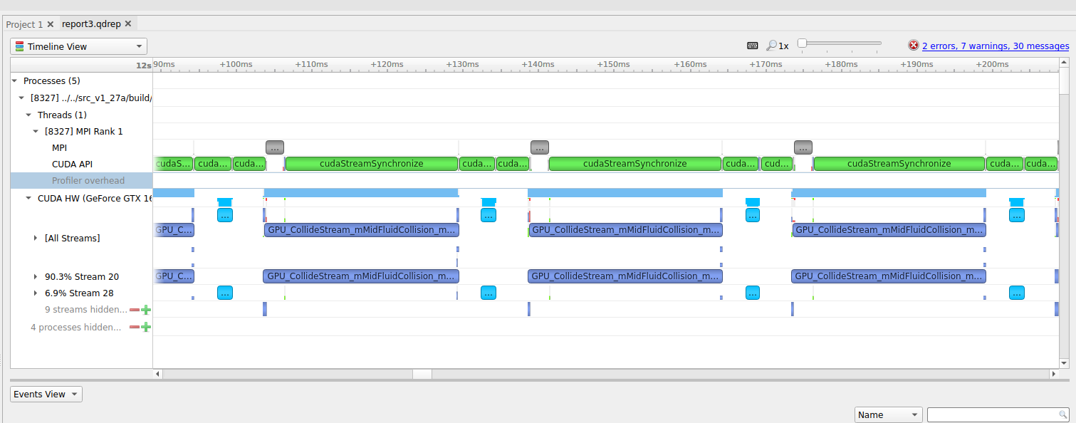
Figure: (a) Profiling HemeLB using NVIDIA Nsight Systems on a laptop. Nsight Systems provides a broad description of the GPU code’s performance (timeline with kernels’ execution, memory copies, cuda streams etc). Focus of analysis in the example here is 3 time-steps of the LB algorithm.

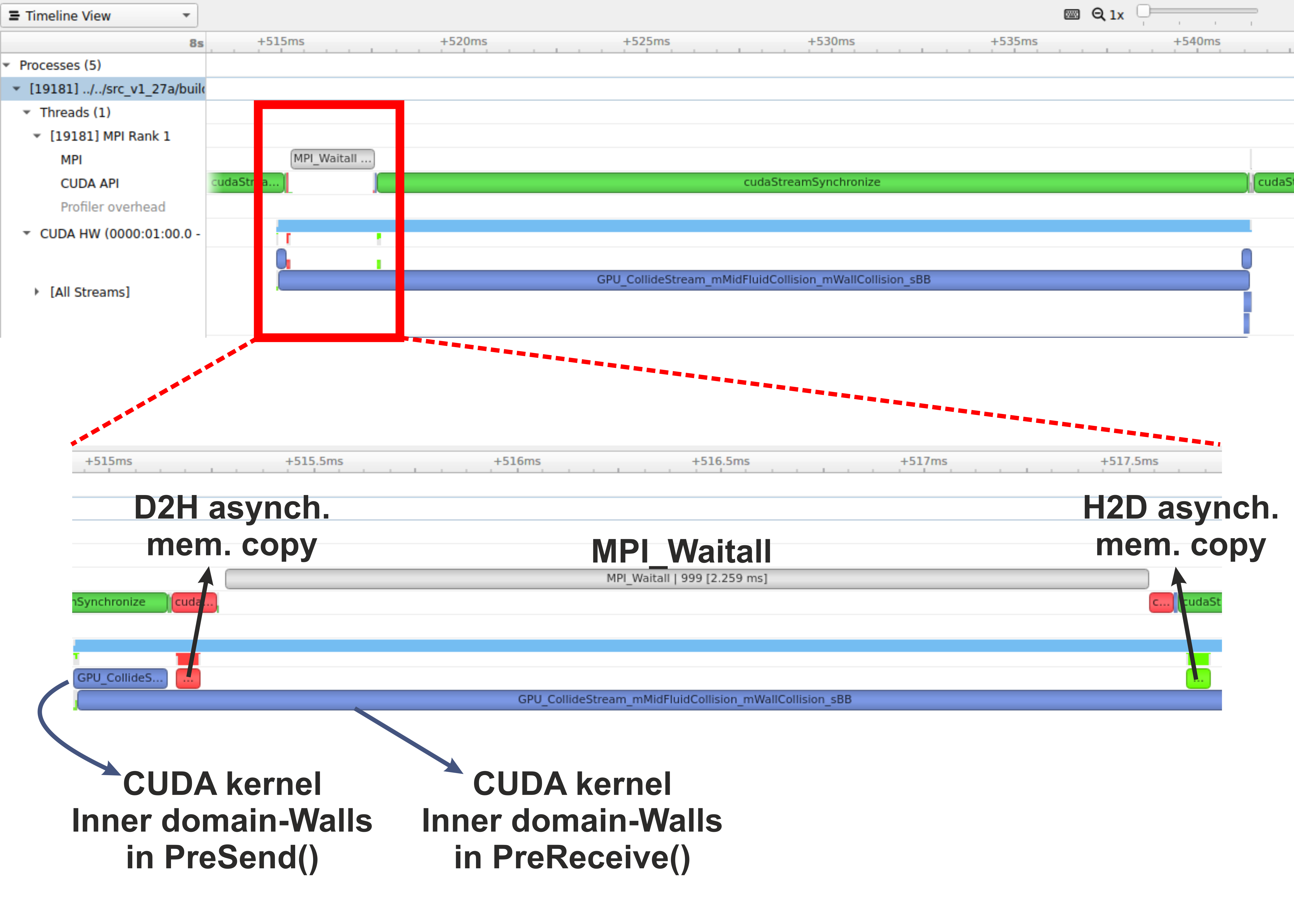
Figure: (b) Profiling HemeLB using NVIDIA Nsight Systems on a laptop. Focus of analysis is 1 time-step of the LB algorithm. Kernels and memory copies overlap during execution on the GPU, as shown in the area marked with the red box.

On a laptop Nsight Systems can be invoked during the CUDA code execution by issuing the following command line:

nsys profile --trace=cuda,mpi,nvtx --stats=true mpirun -np $nCPUs  $PATH_EXE/$EXEC_FILE -in $INPUT_FILE -out results

On HPC systems it may be possible to perform the profiling analysis using Nsight Systems and/or Nsight Compute (see note below).

A note on GPU Profiling

It should be noted that some HPC systems do not readily accommodate GPU profiling tools such as NVIDIA Nsight Systems, owing to that fact that root directory access may be required. You should check with your system administrator of the different options available to you on your system for profiling GPU code.

Running HemeLB on HPC machines with NVIDIA’s GPUs

A GPU accelerated version of HemeLB has been developed using NVIDIA’s CUDA platform. CUDA stands for Compute Unified Device Architecture and is a parallel computing platform and application programming interface model created by NVIDIA. Hence our GPU HemeLB code is GPU-aware; it can only run on NVIDIA’s GPUs.

CUDA does not require developers to have specialised graphics programming knowledge. Developers can use popular programming languages, such as C/C++ and Fortran to exploit the GPU resources. The GPU accelerated version of HemeLB was developed using CUDA C++.

Submitting a HemeLB job on GPUs

When submitting a job script on an HPC machine with nodes containing NVIDIA’s GPUs, the user should specify;

• the number of GPUs to be used on each node
• the specific partition that contains the GPU accelerated nodes.
• the number of MPI ranks
• the number of tasks per node

Run a HemeLB GPU simulation and measure the performance of the code in terms of MLUPS (Millions of Lattice sites Updates per second) per computing core. This can give us a measure of the acceleration achieved by using the GPUs compared to the CPU only simulation.

To enable comparison of the performance of the CPU and GPU versions of HemeLB, use the simulation geometry used in the previous episodes (eg the bifurcation.gmy from episode 3). Try running the GPU code using up to 4 GPUs and report the scaling achieved.

Why do you think a tapering of the performance occurs at the largest GPU counts?

A further testing of the code could be performed by using a bigger simulation domain, so you can use the geometry in files/biggerBif.

Now compare your walltimes for the GPU runs to the CPU version. How many CPUs is your GPU equivalent to?

Using multiple CPUs to access the same GPU

By using multiple CPU cores accessing the same GPU we can speed-up the corresponding part of the work, i.e. the work that needs to be completed on the host (CPU). The work on the device (GPU) should not be affected significantly.

Running a 2-to-1 and 4-to-1 relationship

We could also examine situations where multiple CPU cores (MPI tasks) use the same GPU. This can be achieved by specifying the number of MPI tasks on the nodes being different to the number of available GPUs. For example using the job submission script from Juwels Booster and modifying the following lines.

#SBATCH --nodes=16
#SBATCH --ntasks=128
#SBATCH --ntasks-per-node=8
#SBATCH --partition=booster
#SBATCH --gres=gpu:4

would result in running the simulation with 8 MPI tasks per node and only 4 GPUs per node. This means that we encounter a situation of 2-to-1 CPUs to GPUs.

Provide the timings for running the GPU code using a 2-to-1 and 4-to-1 situation. Report the scaling of the code, as well as the performance (MLUPS per computing core and MLUPS per node, where for the later just divide the performance by the number of nodes used).

Key Points

• Knowing the capabilities of your host, device and if you can use a CUDA-aware MPI runtime is required before starting a GPU run