Accelerating HemeLB

Overview

Teaching: 30 min
Exercises: 90 min

Questions

• What are the various options to accelerate HemeLB?

• What accelerator tools are compatible with which hardware?

Objectives

• Understand the different methods of accelerating a HemeLB simulation

• Learn how to invoke the different accelerator packages across different hardwares

• Understand the risks of trying to naively use HemeLB acceleration methods on a new domain or machine

How can I accelerate HemeLB performance?

There are two basic approaches to accelerate HemeLB simulations that we will discuss in this episode. How successful these will be will depend on the hardware that you have available and how well you know the characteristics of the simulation problem under investigation.

Versions of HemeLB that are accelerated by GPUs are also available and these can yield significant speed-up compared to the CPU code. We will discuss the use of these further in the next episode.

The two options we will discuss in this episode are:

• 1) Vectorisation
• 2) Monitoring

Vectorisation overview

At the heart of many simulation codes will be a relatively small number of kernels that are responsible for the key problem solving steps. In the lattice Boltzmann method of HemeLB it is the update of the fundamental population distributions and the conversion of these to macroscopic properties of interest. When these kernels are written in code, they are often written in variables of the type ‘double’ that may be naively acted on in a sequential manner. However modern processors can operate on multiple ‘double’ sized units of memory at the same time - the latest Intel cores can operate on eight at once. Therefore significant speed-ups can be obtained by invoking parallelism at this fundamental level by adjusting the instructions of this fundamental kernel to allow vector operations. Modern compilers can often do a lot of this without having to write specific code to act in this fashion. However, sometimes code complexity can mean that this is not fully achieved by the compiler and vectorised code needs to be written. This is done through the use of intrinsic instructions that explicitly tell the compiler how a certain portion of code should be compiled.

In HemeLB, the key computational kernels have been encoded with SSE3 intrinsics that allows two ‘double’ units to be operated on simultaneously. This level of optimisation should be compatible with most modern CPUs, even those available on desktops and laptops. To enact this in HemeLB set the -DHEMELB_USE_SSE3 flag in the compilation script to ON and recompile. HemeLB can also use AVX2 intrinsics where the instructions can operate on four ‘double’ units to be acted on with a single instruction. This can be enabled by setting -DHEMELB_USE_AVX2 to ON and the SSE3 flag to OFF. Before trying this, be certain that your CPU is able to use AVX2 intrinsics. The encoding of the key kernels using the intrinsics can be seen in the file src/lb/lattices/Lattice.h. In src/CMakeLists.txt you can identify the compiler flags that are imposed when SSE3 or AVX2 instrinsics are implemented. These options can also allow the compiler to implicitly vectorise some other sections of the code, however the performance of this alone has not been seen to match that obtained when the explicit intrinsics are used for the key computational kernels.

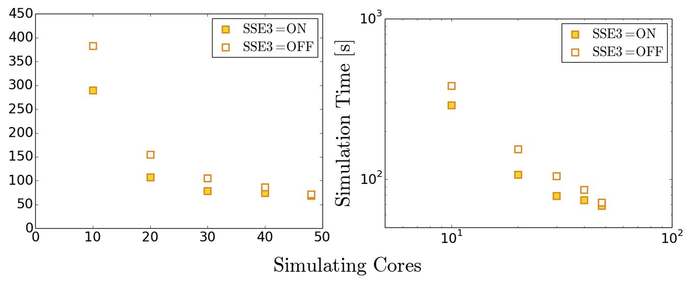
Case Study: Simulation acceleration with intrinsics

Repeat your scaling benchmark tests with SSE3 intrinsics active and compare performance against that achieved with the ‘naive’ code implementation and default compiler options. In particular, note how walltime and parallel efficiency (speed_up_compared_to_smallest/core_scale_up) changes with their use.

Example Results

Note that exact timings can vary between jobs, even on the same machine - you may see different performance. The benefit of using intrinsics can become more apparent at higher core counts, longer runtimes and larger domains.

Scheme	Cores	Initialisation Time (s)	Simulation Time (s)	Total Time (s)
Basic	48	0.7	67.5	68.2
Basic	192	1.0	19.6	20.6
SSE3	48	0.7	56.1	56.8
SSE3	192	1.0	15.2	16.2
AVX2	48	0.7	55.9	56.6
AVX2	192	1.1	14.9	16.0

Monitoring in HemeLB

In the input file provided for the benchmarking case, you will notice the following section:

<monitoring>
<incompressibility/>
</monitoring>

This makes the HemeLB simulation monitor for numerical characteristics that will cause the simulation to become irretrievably unstable and aborts the simulation at this point. This process checks the data at every site in the domain at every time step. As simulation domains grow, this can become a significant portion of the computational time. If you are studying a simulation domain with boundary that are known two generate stable and sensible results, deactivating this feature can reduce the time needed for a simulation to complete. It is STRONGLY recommended to keep this feature active for new domains and boundary conditions to be aware of when simulations are unstable or are possibly on the verge of becoming so. Stability monitoring can be removed by deleting this section or commenting it out via:

<!-- <monitoring>
<incompressibility/>
</monitoring> -->

Case Study: Reduced runtimes without stability monitoring

Repeat the benchmarking tests case for both geometry sizes the with the stability monitoring deactivated. Compare how significant the effect of stability monitoring is for the larger domain.

Another monitoring option that can be introduced to your simulation is a check to observe when steady-state is reached. HemeLB is a explicit solver meaning that it is not ideally suited to steady-state simulations as implicit methods can be. Once a suitable timestep is determined the simulation will continuously step through time until the desired number of iterations is completed. Unfortunately, it is not always possible to know in advance how many iterations are required for steady-state to be reached. This monitoring check will automatically terminate a simulation once a stipulated tolerance value on velocity is reached. This is invoked in the input file by:

<monitoring>
<incompressibility/>
    <steady_flow_convergence tolerance="1e-3" terminate="true" criterion="velocity">
          <criterion type="velocity" units="m/s" value="1e-5"/>
  </steady_flow_convergence> 
</monitoring>

The value for the velocity stated here is the reference value against which the local error is compared.

Case Study: Reduced runtimes for convergence

Repeat the benchmarking test case with the convergence monitoring in place. By how much is the simulation truncated? Try different values for tolerance and input boundary conditions. NB: Steady-state convergence will not work accurately or reliably for intentionally transient flow conditions.

Tuning MPI Communications

Depending on your systems, another option that may yield performance gains is in the modification of how the underlying MPI communications are managed. For general operation however, the default settings provided in the compilation options for HemeLB have been found to work very well in most applications. For the curious reader, the available compilation options are:

Case Study: Demonstration of MPI Setting Choices

To demonstrate the impact of changing MPI options, each were individually examined in turn with all other flags remaining in their default setting. Further discussion on MPI implementation techniques can be found on resources such as https://mpitutorial.com/tutorials/ among many others.

Example Results

Note that exact timings can vary between jobs, even on the same machine - you may see different performance. Here it can be seen that the use of some options in isolation can prevent HemeLB from successfully operating, whilst those with successfult execution only saw variation of performance within the expected variability of machine operation. As an exercise see whether such behaviour is repeated, and occurs consistently, on your local machine.

Scheme	Option	Initialisation Time (s)	Simulation Time (s)	Total Time (s)
All default options	Defaults	0.7	67.0	67.7
-DHEMELB_POINTPOINT_IMPLEMENTATION	'Separated'	0.7	67.3	68.0
-DHEMELB_POINTPOINT_IMPLEMENTATION	'Immediate'	Job Failed	-	-
-DHEMELB_GATHERS_IMPLEMENTATION	'ViaPointPoint'	Job Failed	-	-
-DHEMELB_ALLTOALL_IMPLEMENTATION	'ViaPointPoint'	Job Failed	-	-
-DHEMELB_SEPARATE_CONCERNS	ON	0.7	66.2	66.9

Key Points

• The use of efficiently vectorised instructions can effectively speed-up simulations compared to default options, however they may not be available on all CPUs

• Simulation monitoring in HemeLB can require a significant amount of time to complete. If a set of simulation parameters is known to be stable and acceptably accurate, removal of this feature will accelerate simulation time. It is recommended to be kept in place to catch unstable simulations when new geometries or simulation parameters are being investigated.